Introduction to de Rham Cohomology
Posted: November 23, 2018
Edited: December 15, 2018
Status:
Completed
Categories :
Topology
This post follows Nakahara.
The Name
“de Rham Cohomology” is translated in Chinese as “德拉姆上同调”, where “同调” stands for “the same tune”. I suppose this is related to the musical isomorphism between one forms and vectors. As for the meaning of “co-“, here are my thoughts.
| English | Chinese | Meaning |
|---|---|---|
| cosine/cotangent | 余弦/余切 | adding up to $\pi /2$ |
| coset | 陪集 | dual in the same space |
| cohomology | 上同调 | dual in different spaces |
Body and Boundary
The cohomology is a relationship defined on forms. We will find how to define chains, boundaries, and cycles on differential forms.
The celebrated $\operatorname{d}$
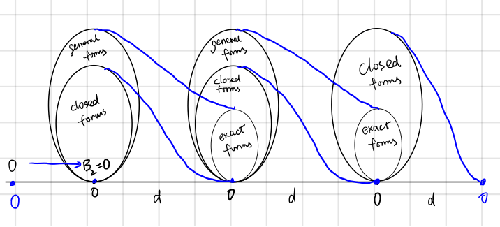
Remember homology relations? It’s very similar to the diagram we found in differential forms and tensors.
\[\begin{array}{cccccccc} &\text{0-forms} & \xrightarrow{\d}{} &\text{$1$-forms} & \xrightarrow{\d}{} & \text{$2$-forms} & \xrightarrow{\d}{}& \text{$3$-forms}&\xrightarrow{\d}{}& 0 \\ &\downarrow &&\downarrow&&\downarrow&&\downarrow \\ &\text{ {functions} } &\xrightarrow{\nabla}{} &\text{ {vector fields} } &\xrightarrow{\nabla\times}{} &\text{ {vector fields} } &\xrightarrow{\nabla\cdot}{} &\text{ {functions} }\\ & function & & divergence & & curl & & gradient \end{array}\]Hence we have the following diagram.
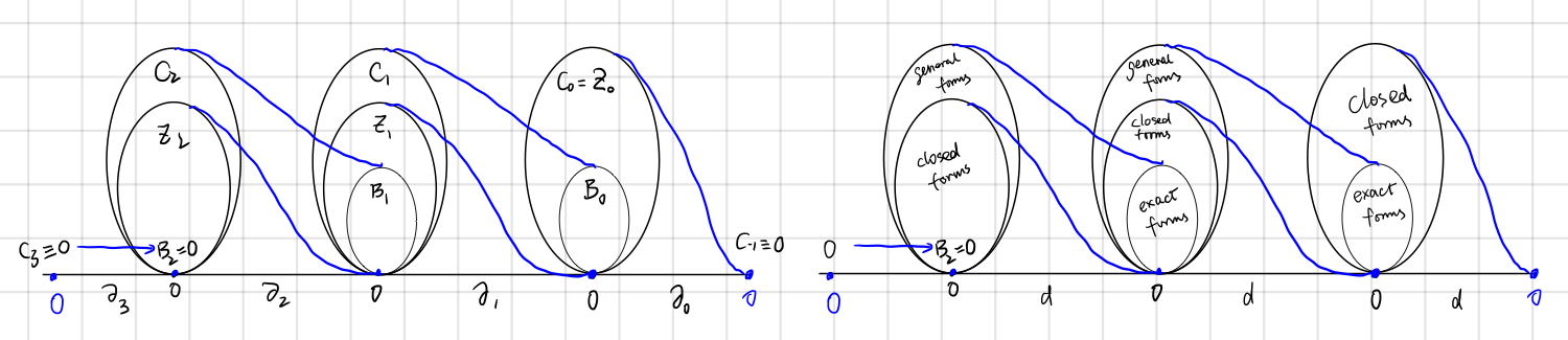
The differences exist but the symbol $\d$ still stands for “take the edge”.
| Homology | Cohomology | Notes | |
|---|---|---|---|
| boundary operator | $\partial $ means “take boundaries” | $\d$ stands for “exterior derivative” | |
| chains | differential forms | ||
| $\d \omega = 0$ | cycle | closed form | “Closed” forms has no boundary, hence the name. |
| $\omega=\d\eta$ | boundary | exact form | Exact forms are “exactly” the exterior derivative of a higher form. |
| $\substack{\d^2=0\newline \partial^2=0}$ | boundaries have no boundary | boundaries have no boundary |
From differential forms, we can tell if a manifold has a whole as we did in homology groups. Still, we need to define the reverse map of $\d$, namely integration, in order to find the $\operatorname{img} 0$.
“Co-“ in Cohomology
As at the beginning of this post, “co-“ means dual, and cohomology group is a dual space of the homology group. This dual relationship is evident in the Stokes’ theorem, as $\partial\leftrightarrow\d$. However, that is not the definition of dual vector space. Like a covector maps a vector to a number, we are looking for this map (i.e., inner product), such that an $r$-chain $c$ and an $r$-from are mapped to a number.
\[c,\omega \mapsto (c,\omega)\in\R\]This map is none other than integration of a differential form over a simplex!.
\[(c,\omega)\dfdas\int_c\omega\]Recall that a simplex of dimension $r$ is defined in $\R^r$ as
\[\sigma _ r=\set{x\in\R^N \mid x=\sum _ {i=0}^n c _ ip _ i, c _ i\ge0, \sum _ {i=0}^n c _ i=1},\]and an $r$-from is now written as
\[\omega=w(\vec x)\, \d x^1 \wedge \d x^2\wedge\cdots\wedge\d x^r\]Integration of a form over a simplex is defined as
\[\begin{align} \int_{\sigma_r}\omega &=\int _{\sigma_r} w(\vec x)\d x^1 \wedge \d x^2\wedge\cdots\wedge\d x^r\\ &\dfdas \nint _{\sigma_r}w(\vec x)\d x^1 \d x^2 \cdots\d x^r \end{align}\]The map is clearly bilinear,
\[(c_1+c_2,\omega)=\int_{c_1+c_2}\omega=\int_{c_1}\omega+\int_{c_1}\omega \\ (c,\omega_1+\omega_2)=\int_{c}(\omega_1+\omega_2)=\int_{c}\omega_1+\int_{c}\omega_2\]Stokes’ Theorem - Duality of $\partial$ and $\operatorname{d}$
We now give Stokes’ theorem without proof in the context of exterior derivative.
\[\int _{\sigma_r} \d \omega = \int_{\partial\sigma _r} \omega\]Example in $3$-dimensional space:
If we take $\omega = a \d x + b \d y + c \d z$, and $w=(a,b,c)$, we have
\[\int_S \vec\nabla\times w \cdot \d \vec S =\oint_C\vec w\cdot\d \vec l\]If we take $\psi=\frac{1}{2}\psi _ {\mu\nu}\d x^\mu \wedge\d x^\nu$, and $F^\mu=\varepsilon^{\lambda \mu\nu } \psi_ {\mu\nu}$, we have
\[\int_V \vec\nabla\cdot \vec F \d V =\oint_S\vec F\cdot\d \vec S\]
It can be written using the bi-linear map as
\[(c,\d \omega)=(\partial c, \omega )\]This duality is in a sense “induces” the homology group and cohomology group.
Definition of the de Rham Cohomology Group
Now with necessary mathematical machinery defined, finally, we will define the cohomology group.
The set of closed $r$-forms on manifold $M$ are called the co-cycle group, denoted $Z^r(M)$, not to be confused with cycle group $Z _ r(M)$. The set of exact $r$-forms on manifold $M$ are called the co-boundary group, denoted $B^r(M)$.
The $r$th de Rham cohomology group is defined as
\[H^r(M)\dfdas Z^r(M)/B^r(M)\]Like in the case of homology group, the cohomology group is just those closed $r$-forms that are not exact.
Exactness
The sufficient and necessary conditions of exactness in the last post about homology are still unanswered.
For a set of cycles $\set{c _ 1, \cdots, c _ k}$ such that $c _ i\not\sim c _ j$, $k=\dim{H_r(M)}$ is the Betti number. A close $r$-from $\omega$ is exact if and only if for all $i=1,2,\cdots,k$
\[\int_{c_i}\omega=0.\]
Make Homology out of Cohomology
So far we have defined the cohomology group and pointed out the relationships between it and the homology group. Now it is time to find some examples.
In short, we are looking for closed $r$-forms that are not exact. For simplicity, we will be looking at one-forms in $2$-dimensional spaces, $\omega = F\d x+G\d y$.
If we take $F$ and $G$ both as polynomials, from $\omega$ is closed,
\[\begin{align*} \d \omega &= \d (F\d x) + \d(G\d y)\\ &=\d F\wedge \d x + \d G \wedge \d y\\ &=\left(\Partial{F}{x}\d x + \Partial{F}{y}\d y \right)\wedge \d x+\left(\Partial{G}{x}\d x + \Partial{G}{y}\d y \right)\wedge \d y\\ &=\left(\Partial{F}{y}-\Partial{G}{x}\right)(\d x \wedge \d y)\\ &=0, \end{align*}\]we have
\[\Partial{F}{y}=\Partial{G}{x}.\]This guarantees the equation
\[\begin{cases} \Partial{f}{x}=F\\ \Partial{f}{y}=G \end{cases}\]has a solution. Which means
\[\d f = \omega\]always hold.
This is interesting. Remember that for $r$-cycles, as long as it is in $\R^3$, it is a boundary. In other words, as long as the manifold has no “holes”, closed forms are always exact. One way to make a hole in the space is to put polynomials in the denominator, for example,
\[\omega=\frac{-y}{x^2+y^2}\d x +\frac{x}{x^2+y^2}\d y\]is closed. However, the manifold now has a hole at $(0,0)$, and it is not exact anymore.
Proof that $\omega$ is not exact:
(From [math stackexchange]) transform $\omega$ in polar coordinates, using \(x = r\cos \theta\notag\\ y = r\sin \theta\notag\)
we have
\[\omega = \d\theta\]Namely, we can define a “function” $f(x,y)=\arctan(y/x)$ such that $\omega=\d f$, and
\[\int_c w = \int_0^{2\pi} dt = 2\pi. \tag{12}\]According to section
Exactness, this form is not exact. That “function” $f$ is not even single value on the entire plane $\R^2/0$.
Now we have applied cohomology theories on trivial spaces and $\R^2/0$, and showed that cohomology can distinguish these two types of spaces. In this sense, cohomology groups serve the same purpose as homology groups: classify spaces in terms of “holes” in it.