---

\[\newcommand{\spl}[1]{\langle{#1}\rangle} \newcommand{\inner}[2]{\left\langle{#1,#2}\right\rangle} \newcommand{\form}{\tilde} \newcommand{\abs}[1]{\left\vert{#1}\right\vert} %\renewcommand{\vec}{\mathbf} \newcommand{\bra}[1]{\left\langle{#1}\right\vert } \newcommand{\ket}[1]{\left| {#1}\right\rangle} \newcommand{\braket}[2]{\left\langle {#1} \; \middle|\;{#2} \right\rangle } \newcommand{\mani}{\mathcal} \newcommand{\field}{\mathscr} \newcommand{\Tspace}[1]{T\! {#1}} \newcommand{\d}{\mathrm{d}} \newcommand{\R}{\mathbb{R}} \newcommand{\D}[2]{\frac{\d {#1}}{\d {#2} }} \newcommand{\Partial}[2]{\frac{\partial {#1} }{\partial {#2} }} \newcommand{\op}{\hat} \newcommand{\uvec}{\hat} \newcommand{\dfdas}{: =} \newcommand{\Eqn}[1]{\text{(Eqn. }\ref{#1}\text{)}} \newcommand{\dual}{\tilde} \newcommand{\vard}{\mathfrak{d}} \newcommand{\vare}{\mathfrak{e}} \newcommand{\e}{\mathrm{e}} \newcommand{\i}{\mathrm{i}} \newcommand{\blue}{\color{blue}} \newcommand{\red}{\color{red}} \newcommand{\norm}[1]{\left\|{#1}\right\|} \newcommand{\set}[1]{\left\lbrace{#1}\right\rbrace} \newcommand{\sgn}{\operatorname{sgn}} \newcommand{\Z}{\mathbb{Z}} \notag\]

Funny Name

I struggled a little for all the terms in Topology meaning “equivalence” (with their even messier Chinese translations: homomorphism (同态), homeomorphism (同胚), isomorphism (同构), homology (同调), homotopy (同伦), isotopy (同痕). Zexian Cao wrote an article in Chinese discussing these strange names, and here is an explanation of homology from Wiktionary. They are not satisfactory as far as I am concerned. I might write an article as soon as I have understood these concepts.

Euler Characteristic

This section follows [Armstrong].

The Counterexample

Euler characteristic is, in fact, a topological invariant. Many of Chinese students encounter this concept around primary school or middle school, as an interesting exercise to develop a sense of space. Nevertheless, it is probably the most famous topological invariant. The law is sometimes stated as Euler’s rule,

Let $V, E, F$ denote the numbers of vertices (corners), edges and faces of a polyhedron respectively, then

\[V-E+F=2\]

Most of the students will draw a few polyhedrons, a cube or a tetrahedron, count these numbers can get the number $2$ and call it a day. However, that is only part of the story. If you try really hard to break the rules, you can come up with at least two more types of “polyhedrons” to prove your teacher wrong.

Name	Image	Vertices $V$	Edges $E$	Faces $F$	Euler characteristic: $V-E+F$
Tetrahedron		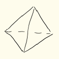4	6	4	2
Cube		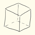8	12	6	2
Cube with a hole (wrong)		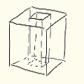16	24	10	2
Cube with a hole (correct)		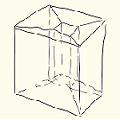16	32	16	0
Hollow cube		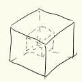16	24	12	4

Notice that a polyhedron’s faces must be simple connected (any two vertices must be connected by an edge), so the correct cube with a hole needs a few extra lines.

You can see that by continuously deforming a cube, to a tetrahedron, Octahedron, Dodecahedron, Icosahedron, you end up with the same number. Once you poke a hole on the polyhedron, the number changes immediately. You can keep deforming continuously until the next hole. The number will remain unchanged. This is the very definition of a topological invariant.

Any quantity We say that this number characterizes the space, hence the name.

Insights of the Counterexample

Why is a cube with a hole different from other polyhedrons and how can we characterize it without using Euler Characteristic?

One way to see it is that it has a hole in it. However, a hole is a concept from daily life, which a typical mathematician might ask unhumorously for clarification. One way to see it is that there exist some loops, as is shown below, that will not cut the surface of this polyhedron into halves. This partly explains the motivation of defining chains and boundaries later.

Triangulation

Homology, however, is just a natural way of defining Euler characteristics in topological spaces. On a side note, it is not the only topological invariant as a “hole-indicator”. The fundamental group and higher homotopy groups will also help to define “holes” on a manifold. This section follows closely [Nakahara].

Triangulation of Objects

Triangulation is again no stranger for anyone who ever took part in IYPT(International Young Physicists’ Tournament), CUPT(China Undergraduate Physics Tournament), or any PTs, and had some experience with COMSOL Multiphysics® software. The following is a triangulation or a “meshing” as is called in the software, of a spring (from Nishant Nath).

It is also very commonly seen at 3D modeling and Art (image from freepik), see also here.

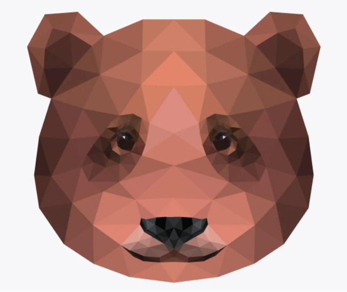
It is self-evident that this technique is very helpful as it converts a smooth object to a “discrete” one while maintaining its most essential traits so that you can still recognize it is a bear. Acute readers might have known where we are heading: we are going to calculate the Euler Characteristic of smooth objects (topological spaces) by triangulating.

Indeed, similar techniques can be adapted to topology spaces. We can use “triangles” to mesh out any oddly shaped topological space, turning it into a “polyhedron”. From this polyhedron, we can calculate the Euler characteristic of the space, telling us how many “holes” are in this topological space. This gives us a way to classify topology spaces according to its “holes”. This is an important aspect of a topological space as in the famous example of topology - a cup and a doughnut is topological equivalent. (image from Wikipedia)

Simplexes

Simplexes are the generalization of triangles and tetrahedrons to lower or higher dimensions. A $0$-simplex, denoted as $\spl{p _ 0}$ is a point, a $1$-simplex $\spl{p _ 0p _ 1}$ is a line, a $3$-simplex $\spl{p _ 0p _ 1p _ 2}$ is a triangle with its interior, a $4$-simplex a solid tetrahedron. A $n$-simplex $\sigma _ n$ is denoted as $\sigma _ n=\spl{ p _ 0,p _ 1,\cdots,p _ n}$, with $\set{p _ i}$ is a set of $n$ geometrically independent points,

\[\sigma _ r=\set{x\in\R^N \mid x=\sum _ {i=0}^n c _ ip _ i, c _ i\ge0, \sum _ {i=0}^n c _ i=1},\quad N\gt n.\]

Informally, an $n$-simplex is the solid polyhedron constructed by $n+1$ points that of the highest dimension.

A simplex can have generalized “faces”. These are named $k$-faces. For instance, a $3$-simplex can have $0$-faces (vertices), $1$-faces (lines), $2$-faces (faces) and $3$-faces (the simplex itself). Since simplex is “simple”, the number of $k$-faces of a $n$-simplex is given by $\binom{k+1}{n+1}=\frac{(k+1)!}{(n+1)!(n-k)!} $.

Simplicial Complexes and Polyhedrons

From simplexes, simplicial complexes can be constructed. Simplicial complexes are again generalizations of polyhedrons in higher or lower dimensions.

A simplicial complex $K$ is a set of simplexes glued together, such that

1. Any face of a simplex of $K$ is part of $K$.
2. Any non-empty intersection of two simplexes belongs to $K$.

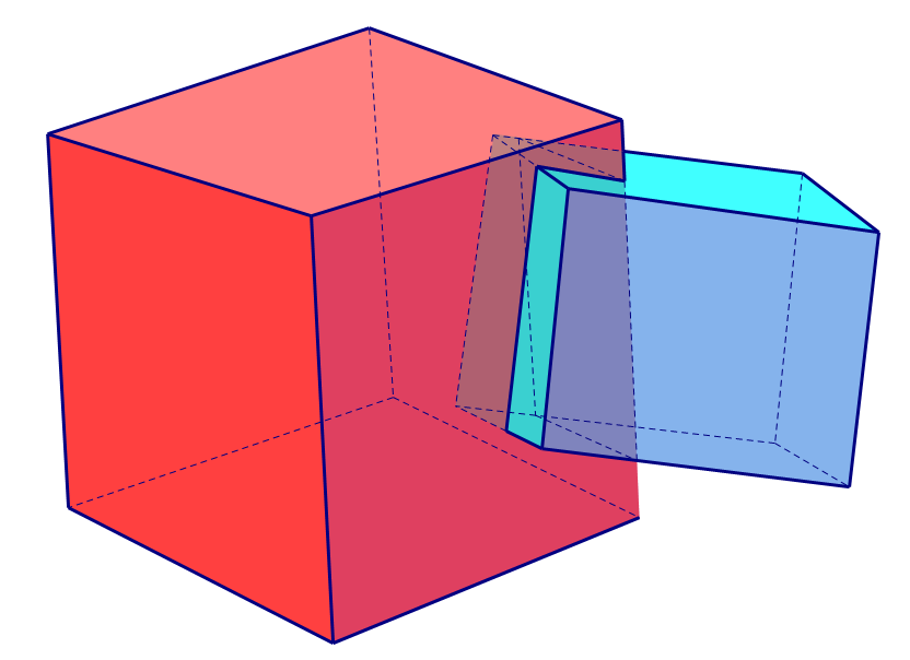
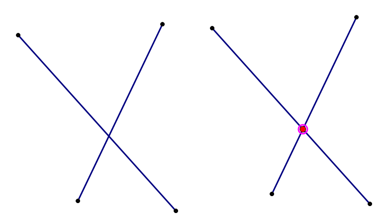
This definition is quite intuitive. By requirement 1., a simplicial complex has a well-defined boundary (surface). All bodies must be covered by a surface. For example, the interior of a cube is not a simplicial complex. By requirement 2., simplexes in a simplicial complex are not allowed to pass through each other freely. By “not passing through”, we mean all the points generated by the intersection must be included. For example, the left is not a simplicial complex for the intersection is not counted while the right is a lawful simplicial complex.

Formally, the simplicial complex $K$ is defined as a set of simplexes.

The dimension of $K$, denoted as $\dim K$ is defined as the largest dimension of simplexes in $K$. This means that although a complex can be in high dimensional space, for example, a triangle embedded in a $4$-dimensional space, the dimension of the complex itself is unchanged, $3$ as in the example.

The set of the above object is

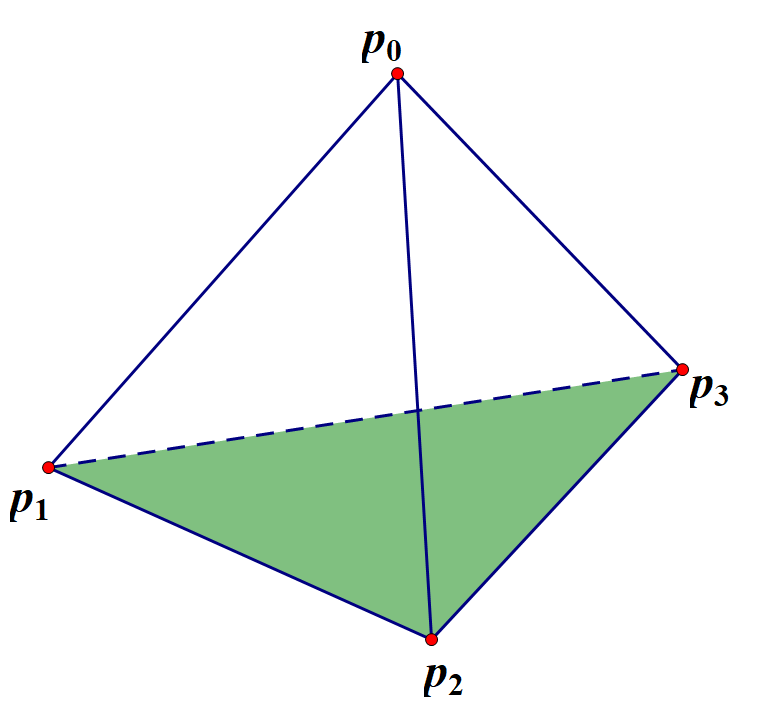
\[\begin{align*} K=\{& p _ 0,p _ 1,p _ 2,p _ 3,\spl{p _ 0,p _ 1},\spl{p _ 0,p _ 2},\spl{p _ 0,p _ 3}, \spl{p _ 1,p _ 2},\spl{p _ 1,p _ 3},\spl{p _ 2,p _ 3},\spl{p _ 1,p _ 2,p _ 3}\} \end{align*}\]

If every simplex in the set is regarded as a subset of $\R^n$, the simplicial complex is called a polyhedron $\abs {K}$.

Triangulation of Topological Space

If there is a homeomorphism $f:\abs{K}\rightarrow X$, topological space is said to be triangulable and the pair $(K,f)$ is called a triangulation.

Homology Group - Elements

From polyhedrons, we are going to construct three groups. By combining these groups, we will be able to find a topological invariant called homology group. This section follows [Nakahara] and [Armstrong].

Oriented Simplexes

The notation of a simplex as $\spl{p _ 1,p _ 2,\cdots,p _ n}$ is in fact insufficient.

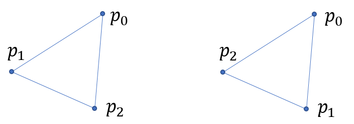
These two triangles cannot be brought to overlap without flipping; neither can these two tetrahedrons without mirroring. Thus for every simplex, we need to define an “orientation”, characterized by the arrangement of the points. It also helps in to define the boundary of simplexes.

\[(p _ {i _ 0},p _ {i _ 1},\cdots,p _ {i _ n})=\sgn (P)(p _ 0,p _ 1,\cdots,p _ n)\]

where

\[P=\begin{pmatrix} 0 & 1 & \cdots & n \\ i _ 0 & i _ 1 & \cdots & i _ n \end{pmatrix}\]

Boundary Operator

The boundary of a complex is of particular interest to us. If we want to calculate the Euler Characteristic somehow, the notions of faces, edges and points are very helpful. They are conveniently the boundaries of bodies, faces, and edges respectively.

The boundary operator $\partial _ r$ acts on an $r$-simplex, and gives its boundary. The $0$-simplex is defined as has no boundary, denoted as $\partial _ 0p _ 0=0$.

Utilizing the orientated simplexes, higher dimensional simplexes can then have well-defined boundaries.

\[\begin{align*} \partial _ r\sigma _ r&=\sum _ {i=0}^{r}(-1)^i(p _ 0,p _ 1,\cdots,p _ {i-1},p _ {i+1},\cdots,p _ r)\\ &\dfdas\sum _ {i=0}^{r}(-1)^i(p _ 0,p _ 1,\cdots,\hat{p _ {i}},\cdots,p _ r)\\ \end{align*}\]

Geometrical examples:

A cube’s boundary is its surface. This surface has no boundary. Similarly, all boundaries have no boundary. Proof see [Nakahara] Lemma 3.3. We will see more about it in section Boundaries.

Note:

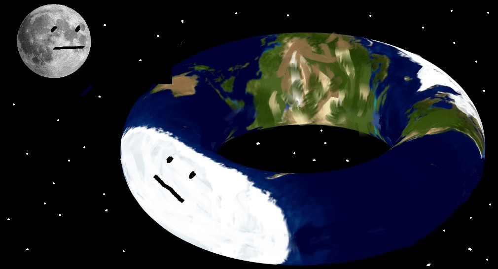
When we say “torus does not have a boundary”, We are talking about the surface.

This may be slightly confusing if you think of torus as the usual “doughnut” hanging in three-dimensional space. However, you should see the doughnut “as it is”, that is to say, only to consider it is own intrinsic geometric structure.

These big words of “intrinsic geometric structure” is still quite hard to understand. Just think of Planet Earth. You are living on the surface of the Earth. You know there are no boundaries on the surface of Earth. Otherwise, Christopher Columbus would have fallen into nothingness.

The same reasoning applies, even if the Earth were a doughnut, you cannot find and boundary to fall from.

Jokes aside, you can think of a sheet of paper as having boundaries, i.e., four edges. Gluing two of them we have a tube, leaving only two edges. Further gluing these two edges together we end up with a torus with no boundaries.

Interlude: Free Abelian Group

An Abelian group is a group whose multiplication is communicative. We then call the group operation “addition”, the identity naturally denoted as $0$.

Example:

​ Integers and addition form an Abelian group.

If every element of an Abelian group $A$ can be written as sum of integer multiples of elements from a subset $\set{G_i}$ of the group $A$. (See a simple definition of a general group generator here.) $A$ is said to be generated by $\set{G_i}$, and elements of $\set{G_i}$ are called generators. If $\set{G_i}$ is also finite, $A$ is said to be finitely generated by $\set{G_i}$.

Example:

• $\Z$ is finitely generated by $\set{1}$ or $\set{-1}$.
• The cycle group $\set{R,2R}$ ($R$ stands for a $180$-degree rotation) is generated by $\set{R}$.
• $\Z\oplus\Z=\set{(m,n)\mid m,n\in Z}$ is finitely generated by $\set{(1,0),\, (0,1)}$ or $\set{(1,0),\,(2,3)}$.

If $\set{G_i}$ is finite, and elements from $\set{G_i}$ are further linear independent, $A$ is called a free Abelian group.

Example:

• The cycle group $\set{R,2R}$ generated by $\set{R}$ is not a free Abelian group, for $R$ is not linear independent. By definition, $R$ is linear independent if $nR=0 \iff n=0$. But for $n=2$, $2R=\text{identity}=0$.
• $\Z\oplus\Z$ is free Abelian group, for it can be generated by $\set{(1,0),\, (0,1)}$, though elements from $\set{(1,0),\,(2,3)}$ are not linear independent.

Examples of Triangulation

It’s always a good idea to base a discussion on some concrete examples. Here are some examples of triangulation on $2$-D manifolds for later use. We went some length to find the simplest triangulations to ensure we are comfortable in later calculations.

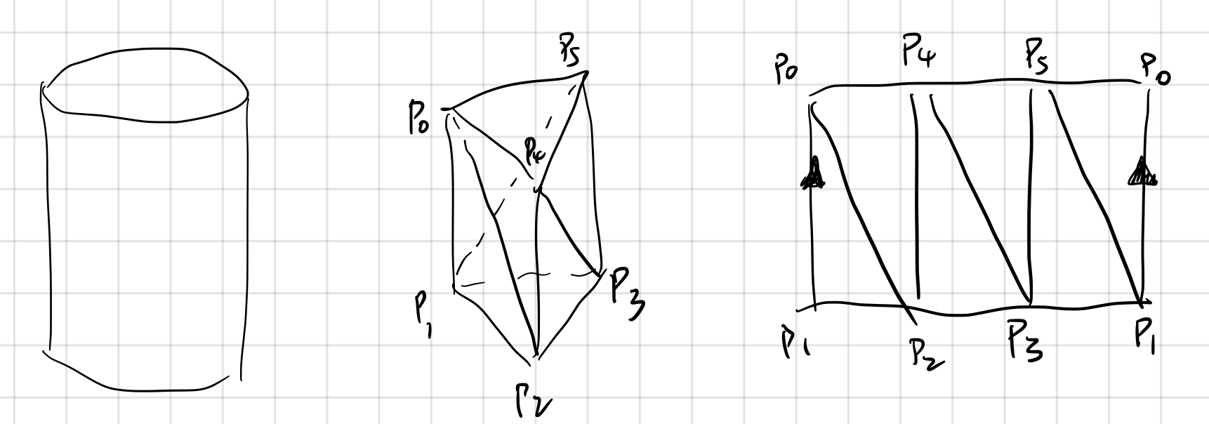
1. Triangulation of the side of a cylinder.

​ The most natural way of seeing the triangulation of a cylinder is to see it as “equivalent” with a triangular prism. However, since the surface of a cylinder is only $2$ dimensional, mathematicians prefer to draw them as flat as possible, so we introduce a notation of “gluing”, as is shown on the right. The arrows on edge $(p _ 0,p _ 1)$ emphasize the way of gluing.

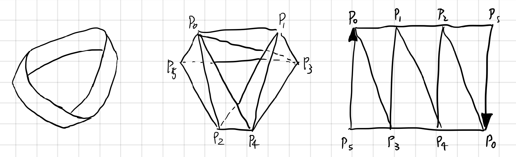
2. Triangulation of the Mobius strip.

​ The famous Mobius strip is much less trivial than the cylinder. Still, we can “crush” the band and see a good way to triangulate it. The arrows on edge $(p _ 0,p _ 5)$ emphasize the way of gluing, as a Mobius strip is made by twisting a strip $180$ degree and then joining the ends of the strip.

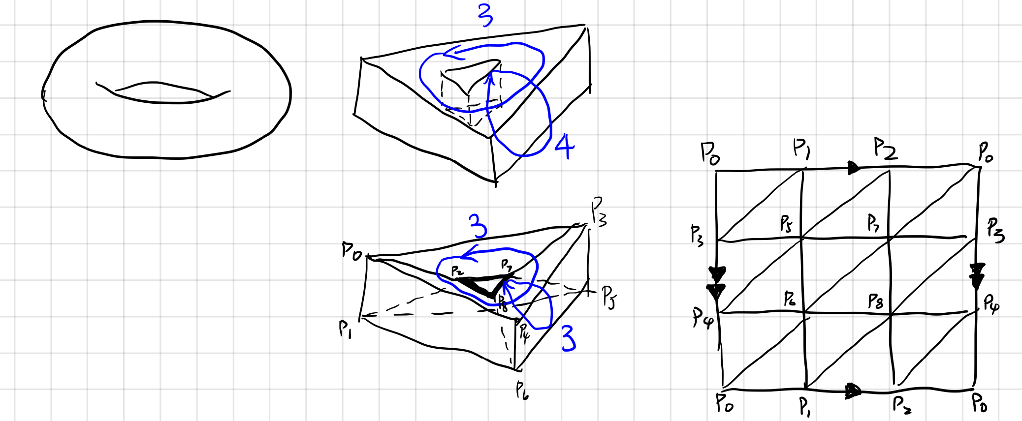
3. Triangulation of Torus.

​ A surface without boundary like a torus can also be conveniently and intuitively triangulated. Note that the simplest triangulation is not a triangular tube. By squeezing the inner upper and lower rim of the tube together, we have a $3\times3$ mesh of triangulation.

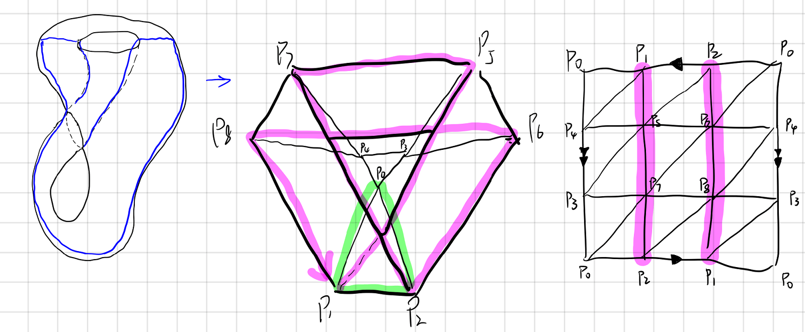
4. Triangulation of the Klein bottle.

​ This page of Klein bottle with animations is an excellent reference if you are unfamiliar with the Klein bottle. In short, a Klein bottle is made by gluing the edge”s” (since there is only one edge) of a Mobius strip. It pieces itself because we are viewing it in $3$ dimensional world. In a $4$-dimensional world, it does not intercept with itself at all.

​ It is quite hard to picture the triangulation of the Klein bottle directly. However, once we know how it is made, we can build it from right to left. The $\color{green}green$ edge is where the piercing occurs. The $\color{magenta} magenta$ line is the “edge” of the Mobius strip.

Chains

Using simplexes from a polyhedron, we can build chains. Like the name suggests, chains are just integer multiples of some oriented $r$-simplexes.

Formally, an $r$-chain is an element of $r$-chain group. The $r$-chain group is the free abelian group generated by every oriented $r$-simplexes of a simplicial complex $K$. A $r$-chain of $r$-chain group is of the form:

\[\sum_{i=1}^{I} n_i\sigma_{r,i},\quad n_i\in\Z\]

The $r$-chain group of simplicial complex $K$ is denoted as $C_r(K)$. We allow $r$ to be greater than $\dim(K)$, by setting all such $C_r$s to be $\set{0}$.

Chain Complex

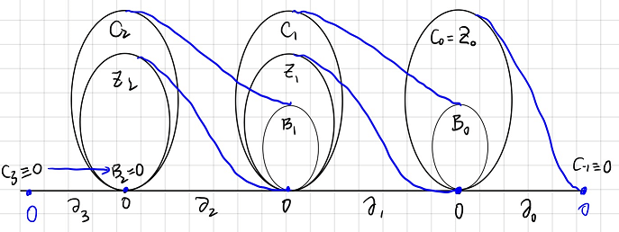
Using boundary operator we can build a chain complex:

\[0\substack{i\\\hookrightarrow}C _ n\xrightarrow{\partial _ n}C _ {n-1}\xrightarrow{\partial _ {n-1}}C _ {n-2}\xrightarrow{\partial _ {n-2}} \cdots\xrightarrow{\partial _ 2}C _ {1}\xrightarrow{\partial _ 1}C_0\xrightarrow{\partial _ 0}0\]

Where $\substack{i \newline \hookrightarrow}$ denotes the inclusion map. Given a subset $B$ of a set $A$, the injection $f:B\rightarrow A$ defined by $f(b)=b$ for all $b \in B$ is called the inclusion map. That is to say:

\[i:0 \rightarrow 0 \in C_n\]

Insisting on putting $0$ on the left side seems to me purely an aesthetic choice. The boundary group $B_n(K) = 0$ is a definition (see Boundaries). This chain complex is commonly seen in k-theories.

Cycles

An $r$-cycle is a chain with no boundary. We can also say that an $r$-cycle $c$ is the kernel of $\partial_r$:

\[\partial_r c = 0\]

All $r$-cycles of $K$ forms $r$-cycle group $Z_r(K)$ (the name is of German origin “Zyklus”). For example, the edge of a triangle and the surface of a torus have no boundary.

Boundaries

An $r$-boundary is an $r$-chain such that it is the boundary of a $(r+1)$-chain. We can also say that an $r$-boundary $b$ is the image of $\partial_{r+1}$:

\[b =\partial_{r+1} c\]

All $r$-boundaries of $K$ forms $r$-boundary group $B _ r(K)$ (“B” stands for “Begrenzung” in German). $B _ {\dim K}$ is defined to be $0$. For example, coincidently, the edge of a triangle, the surface of a torus are boundaries.

Cycles and Holes

You are probably wondering why examples of cycles and boundaries are identical. In section Boundary Operator we know that it can be proven that a boundary can have no boundary. That is to say all boundaries are cycles.

It is natural to ask, are all cycles necessarily boundaries? The answer is No. A trivial example is a single point. A single point has no boundaries but is not a boundary. However, it is hard to come up with an example other than a point. You can draw as many strange shapes as you want, a torus, a two-torus, a torus with a $2$-dimensional fin, etc. However, you will not find such cycles. As a matter of fact, as long as you are drawing in $\R^3$, you will always find your cycle is a boundary of something.

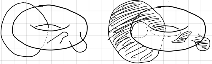
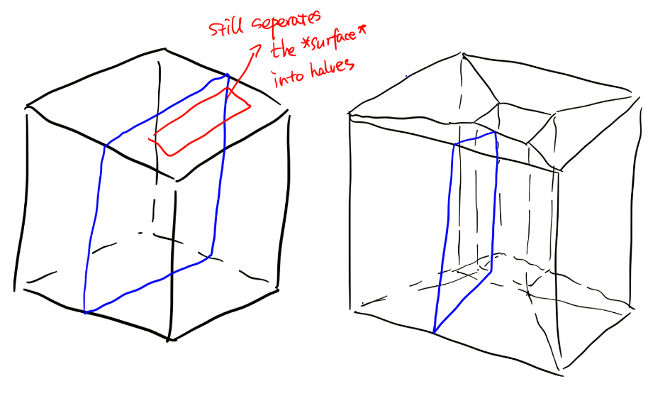
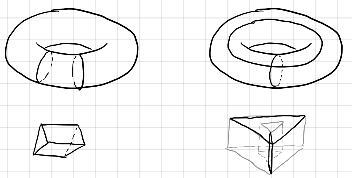
Now let’s study circles on the torus. Are those cycles? Yes. But are those boundaries? One way to see if a cycle is a boundary is to expand the “territory” of the cycle and see if that cycle can contract to a point. You will immediately see the lower two types of cycles are not boundaries of anything.

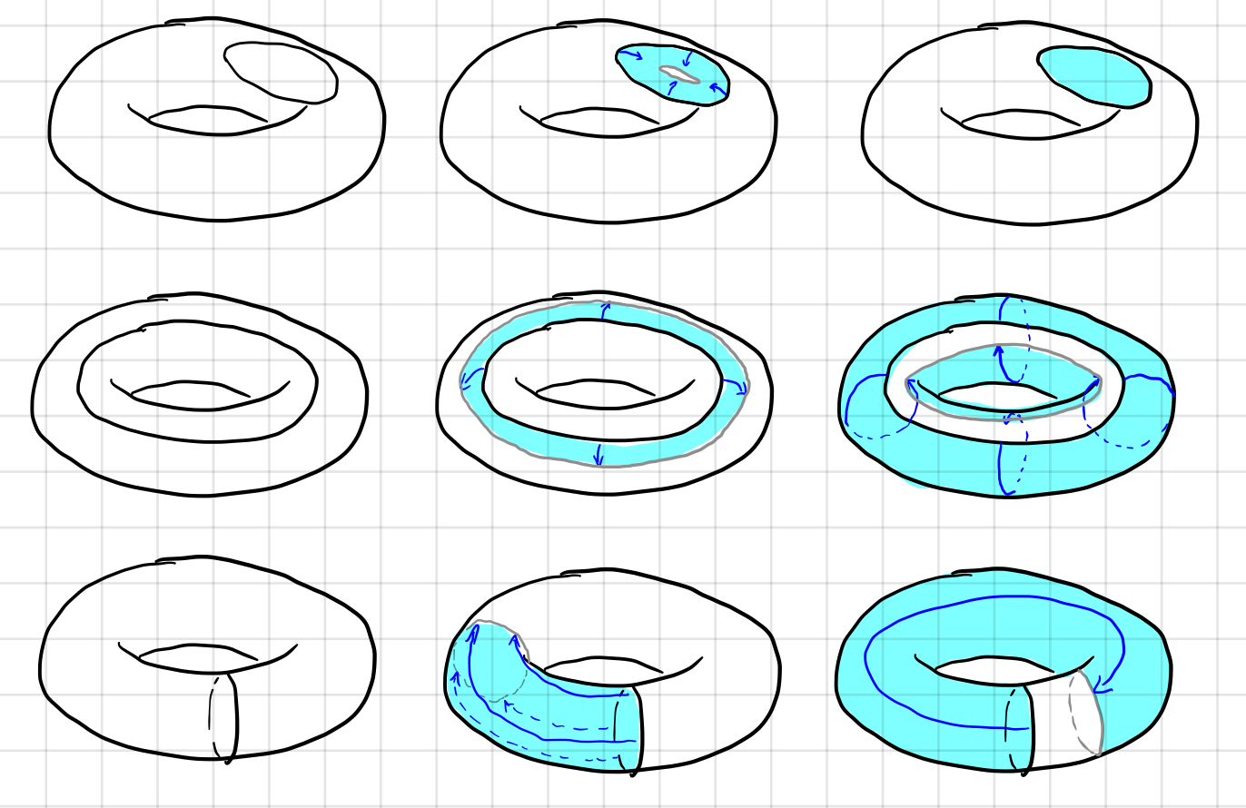
This is the motivation of Homology group. The existence of a cycle that is not a boundary indicates that there is at least one hole on the surface. More information can also be derived using the homology group.

Homology Group

This section follows this paper.

Definition of Homology Group

The chain group $C_r(K)$, cycle group $Z _ r(K)$ and boundary group $B _ r(K)$ of simplicial complex $K$ are obviously not topological invariant. We already know that all boundaries are cycles, but the reverse is not true. Those cycles that are not boundaries are represented by a “division”, i.e., a quotient group. Formally, the Homology group $H _ r(K)$ is defined as

\[H _ r(K)\dfdas Z _ r(K)/B _ r(K).\]

In laymen’s term, Homology group $H _ r(K)$ is the cycles ($Z _ r (K)$) that are not ($ / $) boundaries ($B _ r (K)$).

The notation involves quotient group and equivalent classes. If you are not familiar with those concepts, this reference might help.

Homologous Relation

The Homology group can thus be divided as equivalent classes of cycles \(H _ r(K)\dfdas\set{[z]\mid z\in Z _ r(K)},\)

where

\[[z]=\set{z^\prime\mid z-z^\prime\in B _ r(K)}.\]

If $z$ and $z^\prime$ belong to the same equivalent class, they are called homologous. The two chains on the left are homologous since $z-z^\prime$ is a boundary of a triangular prism $K$, $\dim K=3$. Those on the right are not homologous since $z-z^\prime$ is not a boundary of anything.

Like the discussion in section Cycles and Holes, on the right, $z-z^\prime$ is the boundary of a square and a triangle in $\R^3$, but it’s not a boundary on the torus.

The Euler Characteristic Again

At the beginning of this post, we mentioned defining Euler Characteristic on a smooth manifold. Now it is high time we addressed it from the standpoint of Homology groups. However, I am going to list these theorems without proof simply.

We first treat $Z _ k, \,B _ k,\, H _ k$ and $C _ k$ as vector spaces, and define four numbers as their dimensions as the following:

\[\begin{align} z_k&=\dim (\ker \partial_k),\\ b_k&=\dim (\operatorname{im} \partial_k),\\ h_k&=z_k-b_k,\\ c_k&=\begin{cases}z_k+b_{k-1} \quad &k\gt 0 \\ z_0 &k=0\end{cases} . \end{align}\]

Note a basis for the group of $0$-chains is the set of $0$-simplexes in $K$. The dimension of $C _ 0 (K)$ is, therefore, the number of $0$-simplexes, or the number of vertices $V$. We have $c _ 0 = V$. Similarly, $c _ 1 = E$, $c _ 2 = F$.

Thus the Euler Characteristic can be calculated via

\[\begin{align*} V-E+F&=c_0-c_1+c_2\\ &=z_0-(z_1+b_0)+(z_2+b_1)\\ &=z_0-b_0 -(z_1-b_1)+(z_2-b_2)\\ &=h_0-h_1+h_2 \end{align*}\]

There are much more about homology, but sadly now I will have to move on to Cohomology. Before I go, here are some theorems you might find interesting. There are many notes online if you want to dig deeper.

The Euler-Poincare formula

For all compact, connected surfaces, the Euler Characteristic is $2-h_1$.

Holes and Homology

The number of elements in the equivalence classes of $1$-chains of a surface, i.e., $h _ 1$, is the twice the genus of a surface, where the genus indicates how many holes the surface has.