---

\[\newcommand{\inner}[2]{\left\langle{#1,#2}\right\rangle} \newcommand{\form}{\tilde} %\renewcommand{\vec}{\mathbf} \newcommand{\bra}[1]{\left\langle{#1}\right\vert } \newcommand{\ket}[1]{\left| {#1}\right\rangle} \newcommand{\braket}[2]{\left\langle {#1} \; \middle|\;{#2} \right\rangle } \newcommand{\mani}{\mathcal} \newcommand{\field}{\mathscr} \newcommand{\Tspace}[1]{T\! {#1}} \newcommand{\d}{\mathrm{d}} \newcommand{\R}{\mathbb{R}} \newcommand{\D}[2]{\frac{\d {#1}}{\d {#2} }} \newcommand{\Partial}[2]{\frac{\partial {#1} }{\partial {#2} }} \newcommand{\op}{\hat} \newcommand{\uvec}{\hat} \newcommand{\dfdas}{: =} \newcommand{\Eqn}[1]{\text{(Eqn. }\ref{#1}\text{)}} \newcommand{\dual}{\tilde} \newcommand{\vard}{\mathfrak{d}} \newcommand{\vare}{\mathfrak{e}} \newcommand{\e}{\mathrm{e}} \newcommand{\i}{\mathrm{i}} \newcommand{\blue}{\color{blue}} \newcommand{\red}{\color{red}} \newcommand{\norm}[1]{\left\|{#1}\right\|} \newcommand{\set}[1]{\left\lbrace{#1}\right\rbrace} \notag\]

One form is a concept useful in integration, and the integrand is a one-form. One-form is critical perform integration on Manifold. This post follows Nakahara.

Curves and Functions

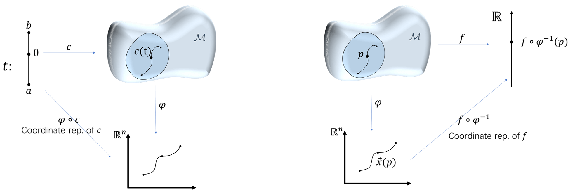
The definitions of curves and functions are as follow. A curve on a manifold is a linear map from interval $[a,b]$ to a set of points. Functions are defined over curves on a manifold, not over curves in $\R^n$. With the help of local coordinates, curves and functions each have coordinate representations.

Vectors and Covectors in Euclidean Space

Vectors

Roughly, a vector space is a set of entities that is closed under linear combinations. Both “arrows” and linear functions satisfy this definition and thus form a vector space.

Due to this remarkable fact, there exists a subset of vectors called the basis in the space, such that any vector in the space can be represented as a linear combination of members of the basis.

A set of basis is denoted as $\uvec e^i$. A vector is then denoted as $V=\sum V ^ i \uvec e _ i$.

Covectors

Now consider the set of linear functions defined on $V$ (vectors) that have values in field $K$ (numbers), i.e. $f:V\rightarrow K$. Such linear functions on vector spaces are called covectors. They are also called linear functionals. They apparently form a vector space $V^*$, since:

• $(f _ 1+f _ 2)(V) = f _ 1(V) + f _ 2(V)$ where the R.H.S. is the addition of two scalars in the field $K$.
• $(kf)(V) = kf(V)$, again where the R.H.S. is the multiplication of two scalars in the field $K$.

The vector space $V^*$ of linear functionals over $V$ is said to be dual to the vector space.

A set of a basis of the dual space is dual vectors as well, which acts on a vector and give a real number. An element of a set of basis is denoted as $\d x ^ i \in \R$. A covector is denoted as $\form \omega=\omega _ i \d x ^ i$.

This suspiciously looking name of the co-basis is carefully chosen for later elaboration, now you can either see it as a derivative $\d$ or merely an abbreviation of “dual”, the real reason for doing this is in section Covectors on Manifold).

The basis’ action on a vector is denoted as $\d x^i (V)$.

Action of Covectors on Vectors

1. Suppose the basis for the vector space $V$ is denoted as $(\uvec x _ 1,\uvec x _ 2, \uvec x _ 3)$, where $\uvec x _ i$ is a unit vector in the positive $x _ i$ direction. Suppose a basis for the dual space $\omega$ is denoted as $(\d x ^ 1,\d x ^ 2,\d x ^ 3)$. From the definition, a basis of a dual space is itself a dual vector, which acts on a vector, gives a real number, i.e., $\d x ^ i(V)\in \R$.

2. Since covectors are linear functionals, $\d x ^ i(V)$ can be seen as an action on bases of vector $V$.

   \[\d x ^ i(V) =\d x ^ i (V ^ 1\uvec x _ 1+V ^ 2\uvec x _ 2+V ^ 3\uvec x _ 3)= V ^ 1\d x ^ i (\uvec x _ 1)+V ^ 2\d x ^ i (\uvec x _ 2)+V ^ 3\d x ^ i (\uvec x _ 3)\in \R\]

3. Define $\d x ^ i (\uvec x _ j)\dfdas \delta ^ i _ j$. We have

   \[\d x ^ i(V) =V ^ j\d x ^ i (\uvec x _ j) = V ^ j \delta ^ i _j = V^i\]

4. The entire action of $\omega=\omega _ i\d x^i $ on vector $V=V^i \uvec x _ i$ is then

   \[\omega (V) =\omega_i \d x ^ i (V) = \omega _i V ^ i\]

Musical Isomorphism

If a vector space is finite dimensional, so is its dual space. In this case, these two linear spaces have the same dimension. Moreover, two linear space of the same dimension are isomorphic (see here).

This isomorphism is relatively simple: swap the basis and nothing changes, $V\leftrightarrow V^*,\, \uvec x _ i \leftrightarrow \d x ^ i$. This isomorphism is called the musical isomorphism. A discussion of the origin of this name can be found here.

This isomorphism is denoted as

\[\begin{align} \sharp : \form \omega \rightarrow \omega^\sharp = W&=\sum(\omega _ \mu \delta ^{\mu\nu})\uvec x _ \nu ,\\ \flat : V \rightarrow V^\flat = \gamma &= \sum(V^\mu \delta _ {\mu\nu})\d x ^ \mu , \end{align}\]

where $\sharp$ is pronounced “sharp”, and $\flat$ “flat”. For $\sharp$ raises the index of components, and $\flat$ lowers the index.

Remark:

• For vector spaces with finite bases the dual spaces are not very exotic; they are essentially the same as the original spaces. There exist some infinite dimensional vector spaces that have dual spaces that are different from the original space.
• For example, Dirac-bras $ \bra{v} $ and -kets $ \ket{v} $ are dual vectors, the contravariant vector $x^\mu$ and covariant vectors $x _ \mu$ are dual to each other. The isomorphisms are both transpose.

Inner Product and Dot Product

The inner product $\inner{\;}{\;}$ is defined as

\[\inner{\omega}{V}=\omega(V) = \omega_i V^i \in\R \label{innerproduct},\]

Note that the inner product is defined between a vector and a dual vector, not between two vectors.

However, the inner product looks suspiciously like dot product. A natural insight is that the dot product of two vectors is a real number, and thus one can “identify” a covector as a vector, inner product as the dot product.

\[\omega(V)=\omega _ i \d x ^ i (V^j\uvec x _ j)=\omega _ i V ^ i=W\cdot V\in \R\]

Gradient and Total Derivative as Duals

It is high time we addressed the weird choice of the name $\d x^i$. We first need a theorem

In Euclidean space, for any vector $V$ there is a non-empty set of functions such that $\set{f \mid \nabla f = V}$.

Proof: Take $f=\sum V^ix^i$. This function belongs to the set $\set{f \mid \nabla f = V}$.

Therefore the gradient of a function $f$ is a vector, denoted as $\vec\nabla f$. Its dual vector is no other than the total derivative of the function $\d f$. The only transition you need is to admit that $\d x^\mu$ can act on a basis vector,

\[\d x^\mu (\uvec x_\nu) = \delta_\nu^\mu. \notag\]

You can check that they fit in the above definition.

\[\begin{align} \d\, f &= \Partial{f}{x ^ \mu} \,\d x ^ \mu\notag\\ \updownarrow\phantom{f}&\phantom{\,} \text{ dual }\phantom{\,=}\updownarrow \label{df-nablaf}\\ \vec\nabla f &=\Partial{f}{x _ \mu}\,\uvec x _ \mu\notag \end{align}\]

Moreover, the action of $\d f$ on a vector $V$ gives the derivative along the direction of that vector, which is a real number.

\[\begin{align} \d f(V)&=\Partial{f}{x ^ \mu}\d x ^ \mu(V)\notag\\ &=\Partial{f}{x ^ \mu}\d x ^ \mu(V^\nu \uvec x _ \nu)\notag\\ &=\Partial{f}{x ^ \mu}V^\nu \d x ^ \mu(\uvec x _ \nu)\notag\\ &=\Partial{f}{x ^ \mu}V^\nu \delta ^ \mu _ \nu\label{df-nablaf-vec-1}\\ &=\Partial{f}{x ^ \mu}V^\mu \notag\\ &=V\cdot \vec \nabla f \label{df-nablaf-vec-2}\\ &\dfdas\nabla _ {V}f=\lim _ {h\rightarrow0}\frac{f(\vec x + hV)-f(\vec x)}{h}\in\R \label{directionalderivative} \end{align}\]

Vectors on Manifolds

We all know what vector is in Euclidean space; a vector is formally defined as an element of a vector space, i.e., a set that is closed under finite vector addition and scalar multiplication.

Though on a manifold, things are a little different. There are three equivalent ways of defining vectors. To put them vaguely,

1. A vector can be represented by an arrow and can be seen as a tuple of numbers;
2. Vector is a (derivation) operator;
3. Vector is an equivalent class of curves (functions).

These definitions are equivalent to each other (proof). So after this chapter, we will make no distinction over these three definitions.

Vector is an arrow

When I think about vector on a manifold, I have the picture of some arrow tangent to the “surface” of a manifold.

Since in general there is no way to define a “straight arrow” connecting two points. Vectors can only be “tangent vectors”. In other words, vectors cannot live on the manifold itself, but the collection of tangent spaces over the entire manifold called the tangent bundle. That way, the vector is kept at a geometrical view. Thus a tangent vector is a generalization of the notion of a bound vector in a Euclidean space.

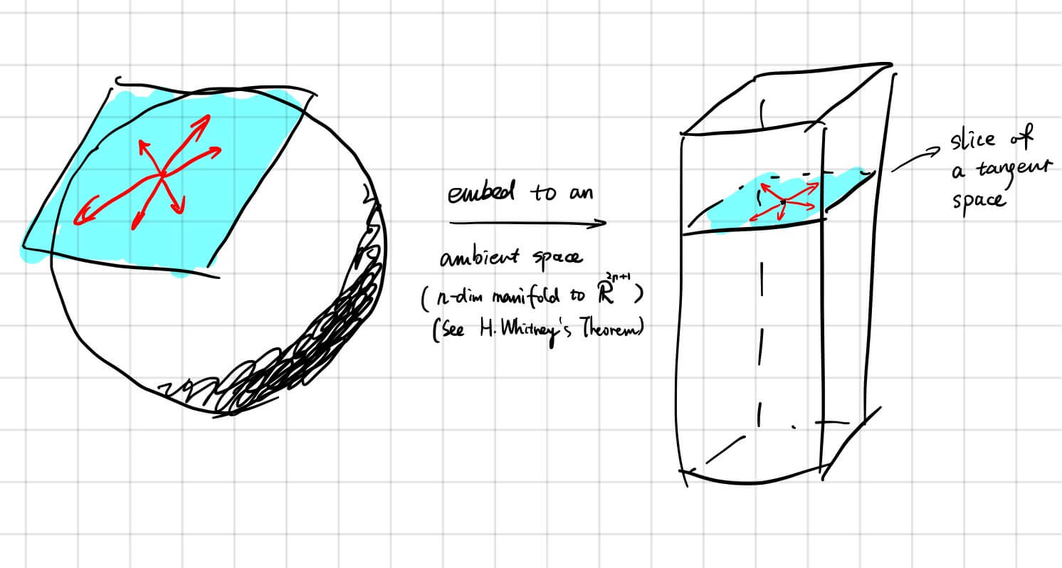
However, this requires embedding the manifold in some higher dimensional space, which is not very convenient since Differential Geometry aims at investigating the space (or maybe space-time) without jumping out of it. Once the vector is in an ambient space, it can be represented by a tuple of numbers. This naïve picture is reasonably intuitive and is mainly brought up as a heuristic way to introduce the next concept.

Vector is a (differential) operator

After I have finished writing this section, I stumbled on [A. Mishchenko and A. Fomenko’s book] and they really excelled at introducing the vectors in a natural way. You should check it out.

The Short Answer

Most of the textbooks only tell you to assign to each vector $V=V^\mu\uvec e_\mu$ an operator $\op V=V^\mu \Partial{}{x^\mu}$. This makes writers happier for there is no further explanation needed - it is just a definition.

How did they come up with it?

Of all the things on a manifold, why did mathematicians choose differential operators?

Because the word “tangent” cries for taking derivatives.

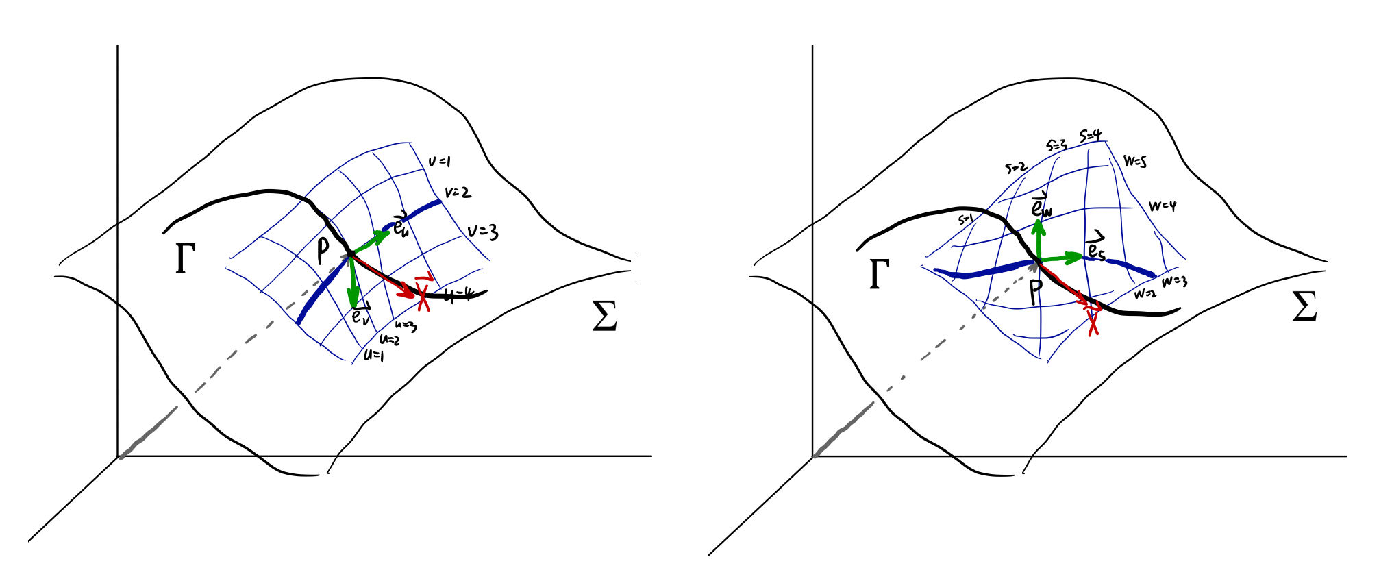
Let’s start with a concrete example: a curved surface $\Sigma :\vec r(x,y,z) = Const$ embedded in $\R^3$. We are going to use this manifold in the context of spacial geometry as a tool to gain some intuition.

On this surface we can have different local coordinates $(u,v)$ (left) or $(w,s)$ (right). For a curve $\Gamma$ on the surface, we can have its coordinates in $xyz$ as $\vec r(t)=(x(t),y(t),z(t))$, or local coordinates as $\vec r(t) = (u(t),v(t))$ or $\vec r(t) = (w(t),s(t))$.

The tangent vector $X$ at $p=\vec r(t _ 0)=(u _ 0,v _ 0)=(w _ 0,s _ 0)$ has a very simple definition in $\R^3 $ as $\vec X = \D{\vec r(t)}{t}$. Using the chain rule,

\[\begin{align} \vec X &= \D{\vec r(t)}{t} \notag \\ &=\left.\Partial{\vec r(u,v)}{u}\right\vert _ {\substack{u=u _ 0\\ v=v _ 0}} \left.\D{u(t)}{t}\right\vert _ {t=t _ 0}+ \left.\Partial{\vec r(u,v)}{v}\right\vert _ {\substack{u=u _ 0\\v=v _ 0}}\left.\D{v(t)}{t}\right\vert _ {t=t _ 0} \notag \\ &=\dot u(t _ 0)\ \left.\Partial{\vec r(u,v)}{u}\right\vert _ {\substack{u=u _ 0\\v=v _ 0}} +\dot v(t _ 0)\ \left.\Partial{\vec r(u,v)}{v}\right\vert _ {\substack{u=u _ 0\\v=v _ 0}} \label{vectorToOperator} \end{align}\]

The expression is now of the form $a \Partial{\vec r}{u}+b \Partial{\vec r}{v}$, with $\Partial{\vec r}{u}$ being an actual $3$-vector.

Next we will see that the term $\Partial{\vec r}{u}$ is independent of choice of curves. If we take the curve $\Gamma$ as $\cases{ u =u(t)\ v =2 }$ in the left figure (or $w=3$ in the right), $\Eqn{vectorToOperator}$ becomes

\[\begin{align} \vec X &= \D{\vec r(t)}{t} \notag \\ &=\left.\Partial{\vec r(u,v)}{u}\right\vert _ {\substack{u=u _ 0\\v=v _ 0}} \left.\D{u(t)}{t}\right\vert _ {t=t _ 0}+0 \notag\\ &=\dot u (t _ 0)\ \left.\Partial{\vec r(u,v)}{u}\right\vert _ {\substack{u=u _ 0\\v=v _ 0}} \label{operator _ basis} \end{align}\]

notice for example, $ \Gamma: \cases{ u=k\cdot t\ v=2} , \vec X =k\left.\Partial{\vec r(u,v)}{u}\right\vert _ {\substack{u=u _ 0\ v=v _ 0}} $ or $ \Gamma^\prime: \cases{u=\tan t\ v=2} , \vec X =\left.\tan(t _ 0)\Partial{\vec r(u,v)}{u}\right\vert _ {\substack{u=u _ 0\ v=v _ 0}}$.

This means if we take a parametrized curve along $v=2$, the tangent vector at point $p$ will always be some number times $ \left.\Partial{\vec r(u,v)}{u}\right\vert _ {\substack{u=u _ 0 \ v=v _ 0}} $ . Thus $\Partial{\vec r}{u}$ is indeed a basis vector independent of curves.

By far, $\Eqn{vectorToOperator}$ means any operator has a component form using differential operators. $\Eqn{operator _ basis}$ means the partial differential operators act like unit vectors or bases of the space of operators. There is nothing we do not already know about differential operators.

What is interesting is how differential operators resemble vectors. They have everything a vector has, namely closedness under linear combinations. From the above example, we can justify that a simple map: $V\rightarrow \op{V} =V\cdot\vec\nabla$ will keep all the properties a vector has, with additional necessary algebraic tools to perform calculations with.

Theorem: The directional derivative of a function defined on the manifold $f(t)$ along the vector $V$ (i.e. tangent vector at $t _ 0$ along the curve $\Gamma(t)$) is the differential operator $\op{V}$ acting on $f$. \(\begin{align} \op{V}(f)&\dfdas\nabla _ {V}f(t)\notag\\ &=\lim _ {t\rightarrow 0}{\frac{f(\gamma(t))-f(\gamma(0))}{t}}\notag\\ &=\lim _ {t\rightarrow 0}{\frac{f(\vec x _ 0+tV)-f(\vec x _ 0)}{t}}\notag\\ \label{vector-as-directional-derivative} \end{align}\)

proof:

\[\begin{align*} \op V (f) &=\left.\D{}{t}f(\Gamma(t))\right\vert _ {\substack{t=t _ 0,\\\text{along }\vec{v}}}\\ &=\left.\D{}{t}f(x^1(t),\cdots,x^n(t))\right\vert _ {\substack{t=t _ 0,\\\text{along }\vec{v}}}\\ &=\sum _ {i=1}^{n}{\dot{x }^i(t _ 0)\Partial{f}{x_i}}\\ \text{notice that } &V =(\dot x^1(t),\cdots,\dot x^n(t)),\vec \nabla f =(\Partial{f}{x_1},\cdots,\Partial{f}{x_n}) \\ &=\vec \nabla f \cdot V\\ &=\nabla _ {V} f \end{align*}\]

Vector is an equivalent class of curves

From above we already know that one can find more than one curve to obtain the same differential operator. If we make a collection of all the curves correspond to the same vector, we can identify a vector with an equivalent class if curves.

Here it goes from Nakahara:

To be more mathematical, we introduce an equivalence class of curves in $\mani M$. If two curves $c _ 1(t)$ and $c _ 2(t)$ satisfy

1. $c _ 1(0) = c _ 2(0) = p$
2. $ \left. \frac{\d x ^ \mu(c _ 1(t))}{\d t} \right\rvert _ {t=0} =\left.\frac{\d x ^ \mu(c _ 2(t))}{\d t}\right\rvert _ {t=0}$

then $c _ 1(t)$ and $c _ 2(t)$ yield the same differential operator $X$ at $p$, in which case we define $c _ 1(t) \sim c _ 2(t)$. Clearly $ \sim $ is an equivalence relation and defines the equivalence classes. We identify the tangent vector $X$ with the equivalence class of curves

\[[c(t)] = \left\lbrace \tilde{c}(t) \mid \tilde{c}(0)=c(0) \text{ and } \left.\frac{\d x ^ \mu (\tilde{c}(t))}{\d t} \right\vert _ {t=0} = \left.\frac{\d x ^ \mu (c(t))}{\d t} \right\vert _ {t=0} \right\rbrace\]

rather than a curve itself.

Vector field

We can assign a vector, say $V$, to each point in the space $X$. This is equivalent to functions of the form $f:X\rightarrow V=(V,\R,+,*)$; i.e., functions which map every point of the space $X$ into the vector space $V$. A vector field can be seen as arrows sprinkled on a manifold as shown in the left. Alternatively, it defines a map from a point to a curve on the manifold as shown in the right.

A point follows the direction of vector field moves at a “velocity” of the magnitude of the vector, tracing out a curve on the manifold.

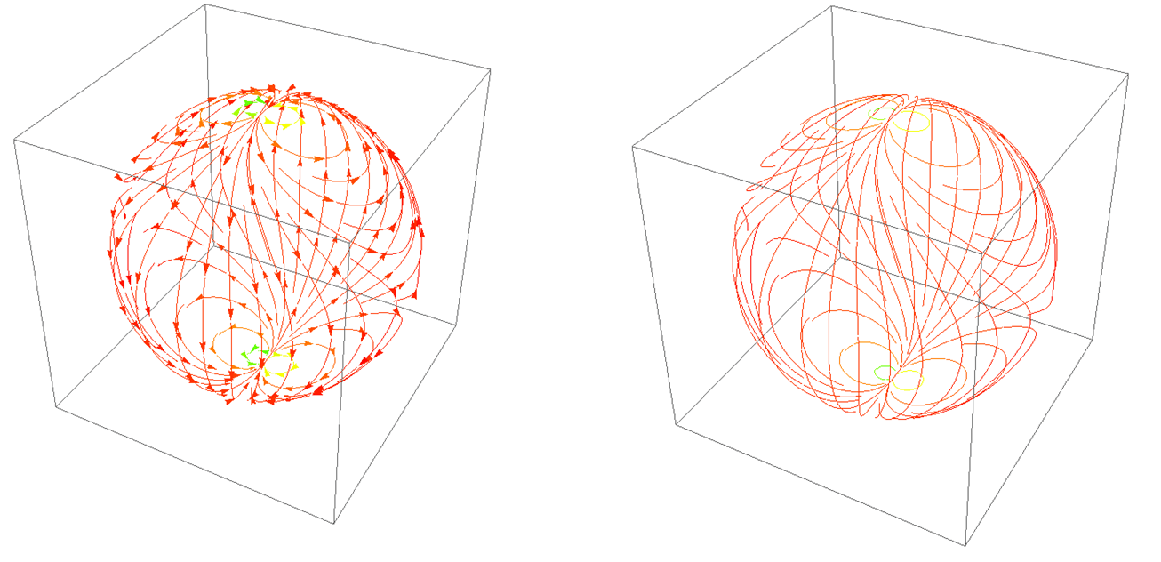
The Lorentz attractor can also be seen as a complicated manifold sprinkled with “velocity vectors.” (from Wikipedia).

One-forms

Covector Revisited

A covector, dual vector, is an element of a dual vector space. On a manifold, it is also called one-form.

A dual vector space is all linear functions that map a vector to $\R^1$. In other words,

A dual vector act on a vector gives a real number.

A dual vector is a linear, real-valued function of vectors.

Covectors on Manifold

Having defined vectors on manifolds, now we are ready to define the dual of vectors.

If one seeks the covector of $V$, he can be equally satisfied asking the question: if the vector $V$ is treated as a covector, what would be the corresponding vector?

Notice that a tangent vector acts on a function gives the directional derivative of that function along the direction of the vector, rewriting $\Eqn{vector-as-directional-derivative}$ with special attention paid to the LHS:

\[\op{v}(f)\dfdas \nabla _ {V}f(t)\in \R.\]

We can also say that a function can somehow act on a vector and gives the directional derivative of the function.

Simply by playing with definitions, we obtain a natural definition of covectors on manifold. To emphasis that, we denote such functions as $\form f$. This is written as \(\form f(V)\dfdas\hat v(f) = \nabla _ V f(t)\in \R.\)

Here are the steps to find the expression for one form $\form f$.

1. To prove the $\form f$ in the above definition form a vector space, i.e., they themselves are vectors.

   This can be verified as following:

   \[\begin{align*} (a \form f+b \form g)(V)&=a \form f(V)+b \form g(V)\\ &=a\nabla _ Vf+b\nabla _ V g\\ &=\nabla _ V(a f+b g) \end{align*}\]

2. To find the basis of this vector space.

   1. First we are going to write down the definition of directional derivative,

      \[\nabla _ {V} f =\sum _ {i=1}^{n}{\left.\D{x ^ i}{t}\right\vert _ {t=t _ 0}\Partial{f}{x^i}} \label{directional-derivative},\]

      with the following identities,

      \[\begin{cases}V =\sum\dot x^i(t)\Partial{}{x^i}\\ d f = \sum \Partial{f}{x^i}\d x ^ i\\ \vec \nabla f =(\Partial{f}{x^1},\cdots,\Partial{f}{x^n})\end{cases}, \notag\]

   2. Now let’s pretend we don’t know the expression of $V$, instead, we are going to try to make up the components of $V$ from the expression by isolating the expression of $f$. The red texts are the components.

      \[\begin{align*} V(f) &= \sum _ {i=1}^{n}{ {\red \left.\D{x ^ i}{t}\right\vert _ {t=t _ 0}}\Partial{f}{x^i}}\\ &=\left(\sum _ {i=1}^{n}{ {\red \dot{x} ^ i(t _ 0)}\Partial{}{x^i}}\right) (f)\\ \end{align*}\]

   3. Following the same procedure, we’ll try to keep the RHS in the form of $(\cdots)(V)$. To do that, first we need an explicit expression of $V$ so we can isolate $V$ later. And we need to insert something else (we call that $\uvec e^i$ for the moment) to maintain the equality.

      \[\begin{align} \form f(V)&= \sum _ {i=1}^{n}{ \left.\D{x ^ i}{t}\right\vert _ {t=t _ 0}{\blue\Partial{f}{x^i}}} \notag\\ &=\sum _ {i=1}^{n}{\blue\Partial{f}{x^i}} \left.\D{x ^ i}{t}\right\vert _ {t=t _ 0}\notag\\ &=\sum _ {i=1}^{n}\left({\blue\Partial{f}{x^i}} \uvec {\mathbf e}^i \right)\cdot \left(\dot x ^ i (t _ 0)\Partial{}{x^i}\right) \label{basis-of-oneform} \end{align}\]

   4. Look at the RHS, we have the form $(X_iY^i)(V)$. Now it’s clear to see that $\uvec e ^ i$ is nothing but the basis of one-form $\form f$, which is also a one form and thus can take $V$ as an input, written as

      \[\begin{align*} \sum _ {i=1}^{n}\left({\blue\Partial{f}{x^i}} \uvec {\mathbf e}^i \right)\cdot \left(\dot x ^ i (t _ 0)\Partial{}{x^i}\right) &=\sum _ {i=1}^{n}{\blue\Partial{f}{x^i}} {\uvec{\bf e}}^i \left(\dot x ^ i (t _ 0)\Partial{}{x^i}\right) \end{align*}\]

      Recall the musical isomorphism

      \[\omega(V)=\omega _ i \d x ^ i (V^j\uvec x _ j)=\left((\omega _ i\delta^{ik})\uvec x_k \right)\cdot\left(V ^ i\uvec x_i\right)=W\cdot V.\]

      we have

      \[\begin{align*} \sum _ {i=1}^{n}{\blue\Partial{f}{x^i}} {\uvec{\bf e}}^i \left(\dot x ^ i (t _ 0)\Partial{}{x^i}\right) &=\sum _ {i=1}^{n}{\blue\Partial{f}{x^i}} {\uvec {\bf e}}^i (V)\\ &=\left(\sum _ {i=1}^{n}{\blue\Partial{f}{x^i}} {\uvec {\bf e}}^i\right) (V) \end{align*}\]

      Where one form $\form f$ is identified as

      \[\form f = \sum _ {i=1}^n\Partial{f}{x^i} {\uvec {\bf e}}^i \notag\]

      where $\uvec e^ i $ is a hungry operator on vectors.

   5. Now the job is to find the exact expression of $\uvec e^ i $. In $\Eqn{basis-of-oneform}$, the basis of one-form was introduced to cancel out the effect of operator $\Partial{}{x^i}$. Putting the context of vectors and covectors aside from now on, just to balance the equation appeared in $\Eqn{basis-of-oneform}$ the product of operator $\uvec e ^ i$ and operator $\Partial{}{x^i}$ in the most conventional sense should be the identity operator. That is to say,

      \[\begin{align*} \left(\uvec{e}^i\Partial{}{x^i}\right) &\equiv 1\\ \left(\uvec{e}^i\Partial{}{x^i}\right) f&\equiv f\\ \uvec{e}^i\Partial{f}{x^i} &= f \end{align*}\]

   6. The answer self-evident,

      \[\uvec e^i =\int \d x^i, \label{basis-one-form}\]

      so that,

      \[\begin{align*} f &\equiv \uvec{e}^i\Partial{}{x^i}f \\ &=\int \d x^i\Partial{f}{x^i} \\ &=f \end{align*}\]

We finally arrive at the conclusion that

\[\begin{align*} \form f = \sum _ {i=1}^n\Partial{f}{x^i}\int \d x^i\\ \form f(V) = \sum _ {i=1}^n\Partial{f}{x^i}\int \d x^i V. \end{align*}\]

Well, that is one boring result. It turns out that this “one form” can be written entirely in the form of integration. It makes great sense if you think of covectors (integration) as counter-parts of vectors (differentiation).

Still, the expression deserves more investigation. Ignoring the context of vectors and covectors, the expression $\Eqn{directional-derivative}$ as function’s derivative show that if two functions $f$ and $g$ have the same differential at $t=t _ 0$,

\[\d f=\sum \Partial{f}{x^i}\d x^i=\d g \notag\]

they will yield the same result,

\[\begin{align*} \nabla _ {V} f -\nabla _ {V} g &=\lim _ {t\rightarrow 0}{\frac{f(\vec x _ 0+tV)-f(\vec x _ 0)}{t}}-\lim _ {t\rightarrow 0}{\frac{g(\vec x _ 0+tV)-g(\vec x _ 0)}{t}}\\ &=\left.\D{}{t}f(x^1(t),\cdots,x^n(t))\right\vert _ {\substack{t=t _ 0,\\\text{along }\vec{v}}}-\left.\D{}{t}g(x^1(t),\cdots,x^n(t))\right\vert _ {\substack{t=t _ 0,\\\text{along }\vec{v}}}\\ &=\D{(f-g)}{t}\\ &=0 \end{align*}\]

In other words, $\form f$ is actually an equivalent class of functions $f$, such that a set of functions $\set{f\mid \d f=\d f _ 0}$, can now be represented as

\[\d f = \sum _ {i=1}^n\Partial{f}{x^i} \d x^i\]

From now on, we will denote one forms as above, instead of $\form f = \sum _ {i=1}^n\Partial{f}{x^i}\int \d x^i$

The Puzzle of $\frac{\partial (dx^\mu )}{\partial x^\nu}$

Now we have made out what vectors and covectors are:

• Vectors are (differential) operators. They are entities of the form

  \[V =\sum a^i\Partial{}{x^i}\]

• Similarly, covectors are entities of the form

  \[\form \omega =\sum a _ i\d x^i\]

So far so good.

The problem rises when you read “A one-form is ‘a thing you plug vectors into’: you feed it a vector and it spits out a number which depends linearly on the input.” You are happy to do some exercises to enhance your understanding of this new concept of covectors. You are smart enough to only use basis of aforementioned vectors and covectors. That gives you

\[\d x^i(\Partial{}{x^j}) =??? \notag\]

Well, that is not clear. You thought maybe if reversing the roles of vector and covector (since they are dual to each other), the result will make more sense. You arrive at

\[\Partial{(\d x^i)}{x^j}=??? \notag\]

That is something you have never seen in calculus, yet it doesn’t look entirely wrong.

Then you turned to a text book for answer, [Sean Carroll] for example. In most (if not all) text books, the equation reads

\[\d x^i(\Partial{}{x^j}) =\Partial{(\d x^i)}{x^j}=\delta _ j^i \notag\]

That can’t be right! You know very clear that $\Partial{x^i}{x^j}=\delta _ j^i$ and $\Partial{(\d x^i)}{x^j}\neq\Partial{x^i}{x^j}$.

A quick google search tells you that these operators are merely “notations”. Another answer went so far as to give the explanation that $\d f$ should be

\[\frac{df}{d} = \frac{\partial{f}}{\partial{x}}\frac{dx}{d} + \frac{\partial{f}}{\partial{y}}\frac{dy}{d}... \notag\]

just to cancel out the $\Partial{}{x}​$.

That bugged me a long time as well. However, if I start from $\Eqn{basis-one-form}$, I know that the basis of “canonical one-form” should be $\int \d x$ rather than $\d x$. We only used $\d x$ to rule out the redundant one forms to establish a one-to-one correspondence. There should be no puzzle anymore since, in some sense, $\d x$ is indeed a notation. And the expression $\frac{d\phi}{d}$ do resemble $\int \d x$ if you think of $\d $ and $\int$ as inverse operations. These two explanations each being only half of the story. Only by combining them can one get a solid understanding of the basis of covectors.

Redefined Vector and One-Forms

At the end of the last section, vectors were generalized as mathematical objects with the form $X=X ^ \mu\Partial{}{x ^ \mu}$. Similarly, the corresponding one-form can be generalized as $\omega = \omega _ \mu \d x ^ \mu$.

This definition will immediately cause a problem: it is no longer guaranteed that a one-form is a total derivative of some function. $x\d y$ is a perfect one-form by this definition, but it is not a total derivative of a function.

This gives rise to exactness and closedness of one-form or $N$-forms.