---

\[\newcommand{\id}{\mathrm{id}} \newcommand{\E}{\mathcal E} \newcommand{\ind}{\mathrm{ind}}\]

Introduction Kitaev’s Model

Remember the term Topological Insulators? I first heard it in my freshman year in a seminar. After his introduction to the system, with lot of terminologies I did not understand, I, being a naïve physics student with folk knowledge in topology, proposed an brilliant idea to the professor: “Will it be interesting if you make the insulator a mobius strip?” The professor clearly did not anticipate that and replied that some of the researcher are doing something like that but the system that he introduced does not exhibit anything new.

Then I learned that most of the times the “topological insulators” are not topological in real space, but in a momentum space. And the concepts are more related to more complicated structures and features, not as simple as “doughnuts and coffee cup” type of topology.

However, there is a model is defined by Kitaev in his paper, where he used square lattice, and he showed that if we consider a 2 dimensional lattice which is a surface of a manifold, it’s ground state degeneracy would depend on the genus of the surface. Meaning that the surface would exhibit real space topology.

My advisor, Dr. Emil Prodan, pushed the results further in his paper to arbitrary triangulations. Some of the triangulation of sphere is listed below.

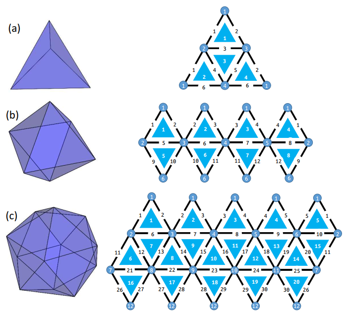
Some of the triangulations of torus is listed below.

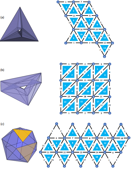
What is interesting is that all the ground state’s degeneracy is independent of actual triangulation, but dependent of the genus of the system.

Definition of the Model

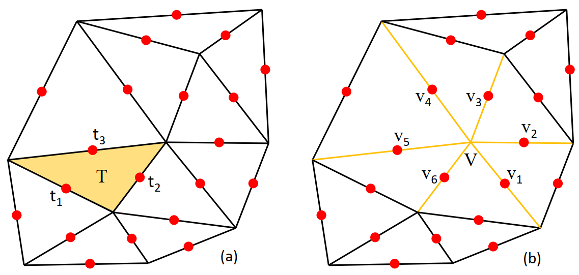
The model is defined on the triangulation, such that on each edge we define two types of operators, $\sigma _ v$ and $\sigma _ t$. On each vertex $v$ we define an operator $A _ v=\displaystyle\bigotimes _ {e \text{ connected to }v}\sigma _ v$, and on each triangle $t$, we define another operator $B _ t=\displaystyle\bigotimes _ {e \text{ constructed by }t}\sigma _ t$.

The Hamiltonian is defined as \(H = -\sum A _ v -\sum B _ t.\) In other words, we want to study the sum over tensor products \(\sum _ {x,y}\id\otimes\id \otimes \cdots \otimes\id\otimes A^x\otimes\id\otimes \cdots \otimes\id\otimes A^y\otimes\id\otimes \cdots \id\otimes\id\)

The tensor product can be grouped as such

\[(\id\otimes\id \otimes \cdots \otimes\id)\otimes A^x\otimes (\id\otimes \cdots \otimes\id) \otimes A^y\otimes (\id\otimes \cdots \id\otimes\id)\]

Analytical Formula

The rule for matrix elements’ tensor product is just

\[E^{(n)} _ {i,j} \otimes E^{(m)} _ {k,l} = E^{mn} _ {(i -1)m+k,(j-1)m +l}\]

The notation $E^{n}$ is to be interpreted as a matrix elements of dimension $n$ by $n$.

Then we have the distributivity of tensor products

\[(A+B)\otimes (C+D) = A\otimes C+A\otimes D+B\otimes C + B\otimes D\]

That means

\[\begin{align} &\id^{n _ 1} \otimes A^{2} \otimes \id^{n _ 2} \otimes A^{1} \otimes \cdots\otimes \id^{n _ K} \otimes A^{Q} \otimes \id^{n _ K+1} \\ &= \left(\sum _ {i _ 1,j _ 1}^{n _ 1} E^{n _ 1} _ {i _ 1,j _ 1}\delta _ {i _ 1,j _ 1} \right)\otimes \left( \sum _ {k _ 1,l _ 1}^{n} A _ {k _ 1,l _ 1} E^{n} _ {k _ 1,l _ 1}\right) \otimes \left(\sum _ {i _ 2,j _ 2}^{n _ 2} E^{n _ 2} _ {i _ 2,j _ 2}\delta _ {i _ 2,j _ 2} \right)\otimes \cdots\\ &= \left(\sum _ {i _ 1,j _ 1}^{n _ 1}\sum _ {k _ 1,l _ 1}^{n} \delta _ {i _ 1,j _ 1} E^{n _ 1} _ {i _ 1,j _ 1}\otimes A _ {k _ 1,l _ 1} E^{n} _ {k _ 1,l _ 1}\right) \otimes \left(\sum _ {i _ 2,j _ 2}^{n _ 2} \delta _ {i _ 2,j _ 2} E^{n _ 2} _ {i _ 2,j _ 2} \right)\otimes \cdots \\ &= \left(\sum _ {i _ 1,j _ 1}^{n _ 1}\sum _ {k _ 1,l _ 1}^{n} A _ {k _ 1,l _ 1}\delta _ {i _ 1,j _ 1} E^{n _ 1n} _ {n(i _ 1-1)+k _ 1,n(j _ 1-1)+l _ 1}\right) \otimes \left(\sum _ {i _ 2,j _ 2}^{n _ 2} \delta _ {i _ 2,j _ 2} E^{n _ 2} _ {i _ 2,j _ 2} \right)\otimes \cdots\\ &= \left(\sum _ {i _ 1,j _ 1}^{n _ 1}\sum _ {k _ 1,l _ 1}^{n}\sum _ {i _ 2,j _ 2}^{n _ 2} A _ {k _ 1,l _ 1}\delta _ {i _ 1,j _ 1} \delta _ {i _ 2,j _ 2}E^{n _ 1n} _ {n(i _ 1-1)+k _ 1,n(j _ 1-1)+l _ 1} \otimes E^{n _ 2} _ {i _ 2,j _ 2} \right)\otimes \cdots\\ &= \left(\sum _ {i _ 1,j _ 1}^{n _ 1}\sum _ {k _ 1,l _ 1}^{n}\sum _ {i _ 2,j _ 2}^{n _ 2} A _ {k _ 1,l _ 1}\delta _ {i _ 1,j _ 1} \delta _ {i _ 2,j _ 2}E^{n _ 1nn _ 2} _ {n _ 2\left(n(i _ 1-1)+k _ 1-1\right)+i _ 2,n _ 2(n(j _ 1-1)+l _ 1-1)+j _ 2} \ \right)\otimes \cdots\\ \end{align}\]

Hence we have

\[\begin{align} &\id^{n _ 1} \otimes A^{2} \otimes \id^{n _ 2} \otimes A^{1} \otimes \cdots\otimes \id^{n _ K} \otimes A^{Q} \otimes \id^{n _ K+1} \\ &= \left(\sum _ {i _ 1,j _ 1}^{n _ 1}\sum _ {k _ 1,l _ 1}^{n}\sum _ {i _ 2,j _ 2}^{n _ 2} A _ {k _ 1,l _ 1}\delta _ {i _ 1,j _ 1} \delta _ {i _ 2,j _ 2}E^{n _ 1nn _ 2} _ {n _ 2\left(n(i _ 1-1)+k _ 1-1\right)+i _ 2,n _ 2(n(j _ 1-1)+l _ 1-1)+j _ 2} \ \right)\otimes \cdots\\ &= \left(\sum _ {i _ 1}^{n _ 1}\sum _ {i _ 2}^{n _ 2} \sum _ {k _ 1,l _ 1}^{n}A _ {k _ 1,l _ 1}E^{n _ 1nn _ 2} _ {n _ 2\left(n(i _ 1-1)+k _ 1-1\right)+i _ 2,n _ 2(n(i _ 1-1)+l _ 1-1)+i _ 2} \ \right)\otimes \cdots\\ &= \left(\sum _ {i _ 1}^{n _ 1}\sum _ {i _ 2}^{n _ 2} \sum _ {k _ 1,l _ 1}^{n}\sum _ {k _ 2,l _ 2}^{n}A _ {k _ 1,l _ 1}A _ {k _ 2,l _ 2}E^{n _ 1nn _ 2n} _ {n(n _ 2\left(n(i _ 1-1)+k _ 1-1\right)+i _ 2-1)+k _ 2,n(n _ 2(n(i _ 1-1)+l _ 1-1)+i _ 2-1)+l _ 2} \ \right)\otimes \cdots\\ &= \left(\sum _ {i _ 1}^{n _ 1}\sum _ {i _ 2}^{n _ 2} \sum _ {i _ 3}^{n _ 3} \sum _ {k _ 1,l _ 1}^{n} \sum _ {k _ 2,l _ 2}^{n} A _ {k _ 1,l _ 1}A _ {k _ 2,l _ 2}E^{n _ 1nn _ 2nn _ 3} _ {n _ 3(n(n _ 2\left(n(i _ 1-1)+k _ 1-1\right)+i _ 2-1)+k _ 2-1)+i _ 3,n _ 3(n(n _ 2(n(i _ 1-1)+l _ 1-1)+i _ 2-1)+l _ 2-1)+i _ 3} \ \right)\otimes \cdots\\ \end{align}\]

We can see that the indices of $E$ are

\[i _ 1\\ n(i _ 1-1)+k _ 1\\ n _ 2(n(i _ 1-1)+k _ 1-1)+i _ 2\\ n(n _ 2(n(i _ 1-1)+k _ 1-1)+i _ 2-1)+k _ 2\\ n _ 3(n(n _ 2(n(i _ 1-1)+k _ 1-1)+i _ 2-1)+k _ 2-1)+i _ 3\]

organizing the last term,

\[\begin{align} &n _ 3(n(n _ 2(n(i _ 1-1)+k _ 1-1)+i _ 2-1)+k _ 2-1)+i _ 3\\ &=n _ 3nn _ 2ni _ 1+n _ 3nn _ 2k _ 1+n _ 3ni _ 2+n _ 3k _ 2+i _ 3-n _ 3nn _ 2n-n _ 3nn _ 2-n _ 3n-n _ 3\\ &=n _ 3nn _ 2n(i _ 1+n^{-1}k _ 1-1-n^{-1})+n _ 3n(i _ 2+n^{-1}k _ 2-1-n^{-1})+i _ 3\\ \end{align}\]

we know from induction,

\[\begin{align} \ind(i,k)&=\sum _ {r=1}^{Q}\left(\prod _ {s=Q}^{r+1}n _ s n\right)i _ r +\sum _ {r=1}^{Q}\left(\prod _ {s=Q}^{r+1}n _ s n\right)n^{-1}k _ r -\sum _ {r=1}^{Q}\left(\prod _ {s=Q}^{r+1}n _ s n\right)(1+n^{-1}) \\ &=\sum _ {r=1}^{Q}\left(\prod _ {s=Q}^{r+1}n _ s n\right)(i _ r+n^{-1}k _ r-1-n^{-1}) \\ &=\sum _ {r=1}^{Q}\left(\prod _ {s=Q}^{r+1}n _ s n\right)(i _ r+(k _ r-1)/n-1) \end{align}\]

Then we can find

\[\underbrace{\sum _ {i _ 1}^{n _ 1}\sum _ {i _ 2}^{n _ 2}\cdots \sum _ {i _ {Q+1}}^{n _ {Q+1}}} \underbrace{\sum _ {k _ 1,l _ 1}^{n}\cdots \sum _ {k _ K,l _ K}^{n}} A _ {k _ 1,l _ 1}A _ {k _ 2,l _ 2}\cdots A _ {k _ Q,l _ Q} E^{n^{Q}n _ 1n _ 2\cdots n _ Q} _ {\ind(i,k),\ind(i,l)}\\\]

The codes for one configuration

The code would be

The problem of the above code is that the number of non-trivial operators $Q$ is hard coded and cannot be changed by simply changing $Q=Q+1$.

Possible problems of the codes

The code is too deep

The above code for generating one term of the Hamiltonian needs to be put inside of a loop for generating “configurations” of $n _ i$’s, resulting the loop being too deeply nested.

This can be solved by

The number $Q$ is hard-coded

The loop

Solution

The two above problems can be solved by replacing the nested loops to a “smart conversion”.

The idea is to convert the total loop $n^{L-Q}$ to a number such that it’s $i$th digit is of base $n(i)$, or better,

\[n^{L-Q} \rightarrow \overline{i(Q+1) _ {\scriptsize n(Q+1)}\cdots i(2) _ {\scriptsize n(2)} i(1) _ {\scriptsize n(1)}}\]

The loop over $i()$’s can be replaced by

The loop over $k$ and $l$ will be easily modified in the same way.

Combined Codes

Possible enhancements

• The outmost loop contains a lot of unwanted loops. When $Q$ is small compared to $L$, there are bound to be a lot of wasted resources and jumps. If the go to statements breaks the parallelization, we can relabel the qualified loopn’s and write that into a much smaller loop.
• In extreme case, we can even compress the entire nested loop into one single big loop using the techniques stated above. But that might result in a code that is hard to understand.
• In each loop, the product of $A$ is constructed more times than needed.

Publication and Improved Code Samples

The final optimal codes is published on arXiv:1912.12964 with many examples.