---

\[\newcommand{\bra}[1]{\left\langle{#1}\right\vert } \newcommand{\ket}[1]{\left\vert {#1}\right\rangle} \newcommand{\braket}[2]{\left\langle {#1} \, \middle\vert \,{#2} \right\rangle } \newcommand{\uvec}{\hat} \newcommand{\dfdas}{:=} \newcommand{\Eqn}[1]{\text{Eqn. (}\ref{#1}\text{)}} \newcommand{\set}[1]{\left\lbrace {#1}\right\rbrace} \newcommand{\vac}{ {1\!\!1}} \newcommand{\la}{\mathfrak} \newcommand{\anti}{\overline} \newcommand{\Id}{\mathbb I} \newcommand{\e}{\mathrm{e}} \newcommand{\xeq}[1]{\substack{\text{#1}\newline =}} \newcommand{\rc}{\dashv} \newcommand{\lc}{\vdash} \newcommand{\ints}{\mathbb{ Z}} \newcommand{\Reals}{\mathbb{R}} \newcommand{\Hashtag}{\rlap{=}/\!/} \newcommand{\hashtag}{\mathchoice{\Hashtag}{\Hashtag}{\scriptsize\Hashtag}{\tiny\Hashtag}} \require{cancel} \notag\]

This post mostly follows ¹.

Overview of the Strangeness of Knots Theory

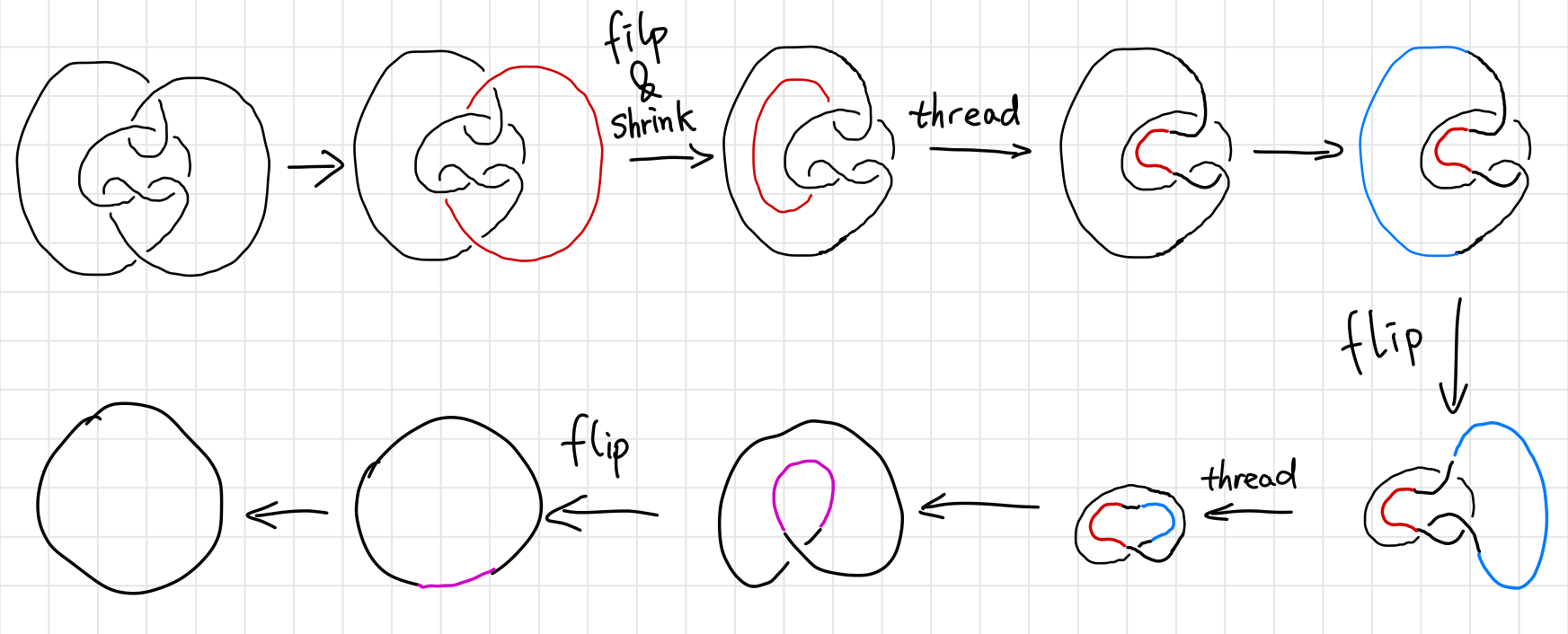
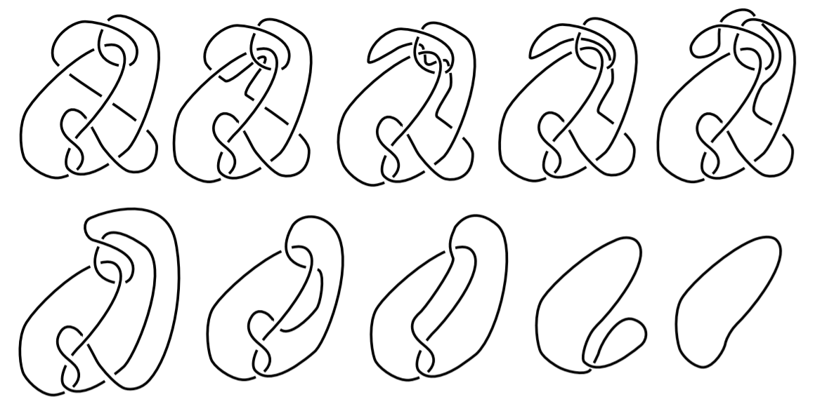
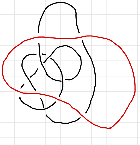
Knots are simple and mundane objects everyone knows from their daily life. Tying is easy and untying a knot can be challenging. What is more challenging is to tell if a knot is “the same” as another one, namely the classification of knots. As is shown by the magic tricks in the beginning of Dr. Kauffman’s lecture at KITP titled Revolutions in Knots, Braids and Physics, Louis Kauffman, our intuition can not be trusted. Below is an example of a nasty unknot (Example taken from²).

The first thing is the introduction of polynomials to the knots. Since the study of knots and its deformations are clearly in the realm of topology, we seek topological invariance to characterize knots. In other words, we assign an entity (not necessarily a quantity) to each knot. If two knots are assigned to different entities, then they are not the same. As some might have known, such entities can emerge in the form of a simple number (Chern number), or a group (Homology groups), which are quite straight forward to understand. I mean, topology is about deformation and transformation, and I understand that you can assign a group to a manifold to characterize its symmetry etc. But what does a polynomial - not a polynomial appeared in an equation such as $x^2-2x+1=0$, but a dangling, lonely polynomial $x^2-2x+1$ - has to do with knots?

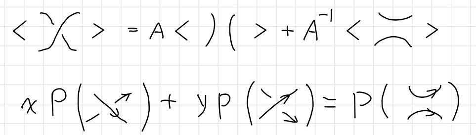
The second thing, which is even weirder, is that to calculate (some) polynomials, equations looks like doodles are introduced. Such equations are “defined”, as is pointed out by a good number of textbooks, which is simply beyond me. First of all, how am I supposed to read the equation? Two crossing arcs is the sum of two different configurations of non-intersecting arcs? Second of all, what does the bracket doing in the equation? Should I interpret the equation as some sort of superposition? Is a knot a quantum state that can be superposed or is it an observable that can be sandwiched by state vectors? What are these state vectors?

Such questions haunts me when I was reading Pachos’ book of TQC, and other books in TQC doesn’t seem to be of much help either. “This is the definition”, as is always the case when something is hard to explain. I spent a good half of a day trawling the introductory materials in mathematics departments I could find on Google, and I think I have a good answer to the questions above.

Naïve Knot Theory

“Strings” Theory in 1867

In 1860s, Lord Kelvin, like all giants in science, was pondering about a theory that could explain

• The stability of atoms.
• The variety of atoms, as shown by the periodic table of elements.
• The vibrational properties of atoms, as shown by their spectral lines.

One day he saw smoke rings of his physicist friend P.G. Tait³, and was impressed by their stability, and vibrational properties of the smoke rings. He noticed how knots resembles atoms in many ways. In 1867, He presented a paper to the Royal Society of Edinburgh, in which he wrote:

Models of knotted and linked vortex atoms were presented to the Society, the infinite variety of which is more than sufficient to explain the allotropies and affinities of all known matter.

Lord Kelvin’s envision of atoms as tiny knots vortices of ether (like a knotted smoke ring, which has only been recently realized in lab⁴) is a very insightful discovery, since it’s not that far from what we call string theory today, which envisions fundamental particles as vibrating strings.

Definition:

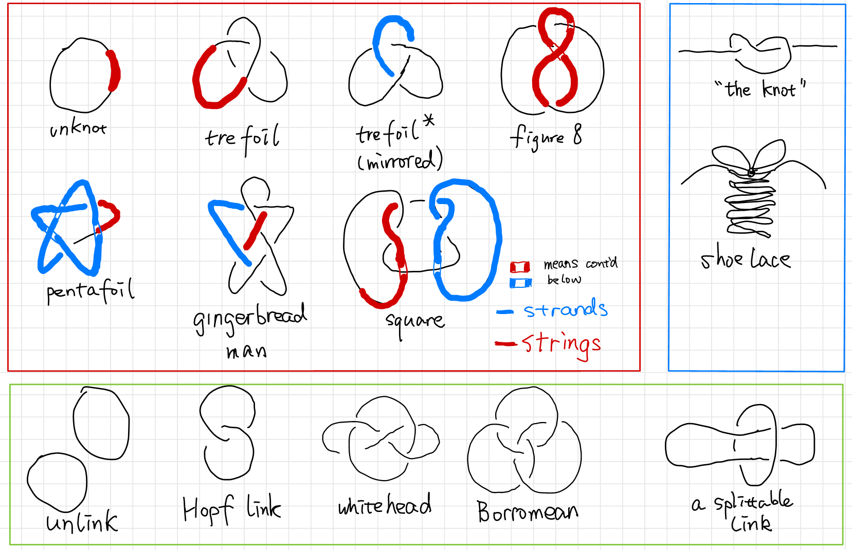
A knot is an entangled string with no open ends. A knot consists of a single string. A link consists of multiple strings. In this post these two words may be used interchangeably since how many strings are there is rarely our concern. A strand is a piece of the link that goes from one undercrossing to another with only (zero or more) overcrossings in between. The word “string” is reserved as a general pronoun for the mathematical abstraction of a rope.

A knot is drawn on a $2$ dimensional paper as a projection of a $3$ dimensional objects. In such projections, a crossing can only be produced from two strands, since we can always move away strands in a crossing with three or more strands.

So Tait decided to find a “table of knots” and compare to Mendeleev’s “table of elements”. So he did. He made little progress with the enumeration problem until the start of a happy collaboration with Little and Kirkman. Tait spent 10 years of work on his list of knots and got up to 10 crossings. The work gets increasingly hard as there are more and more “crossings” on a knot. It’s hard to tell if two knots are the same. He came up with a crossing index, which is the minimal crossings of a knot’s planar projection. The crossing index is by definition a knot invariant. If two knots have different crossing number they are not the same.

History from⁵,⁶,⁷.

Reidemeister’s Moves

The vortex theory of the atom soon disappeared, and physicians lost interests in the mathematical theory of knots, but mathematicians found the knots intrinsically beautiful objects to study and continued develop the theory independent of physical interest.

Now it’s interesting that the circle closes in the last decades for knots theory become very important in physics again due to it connection with QFT and string theory.

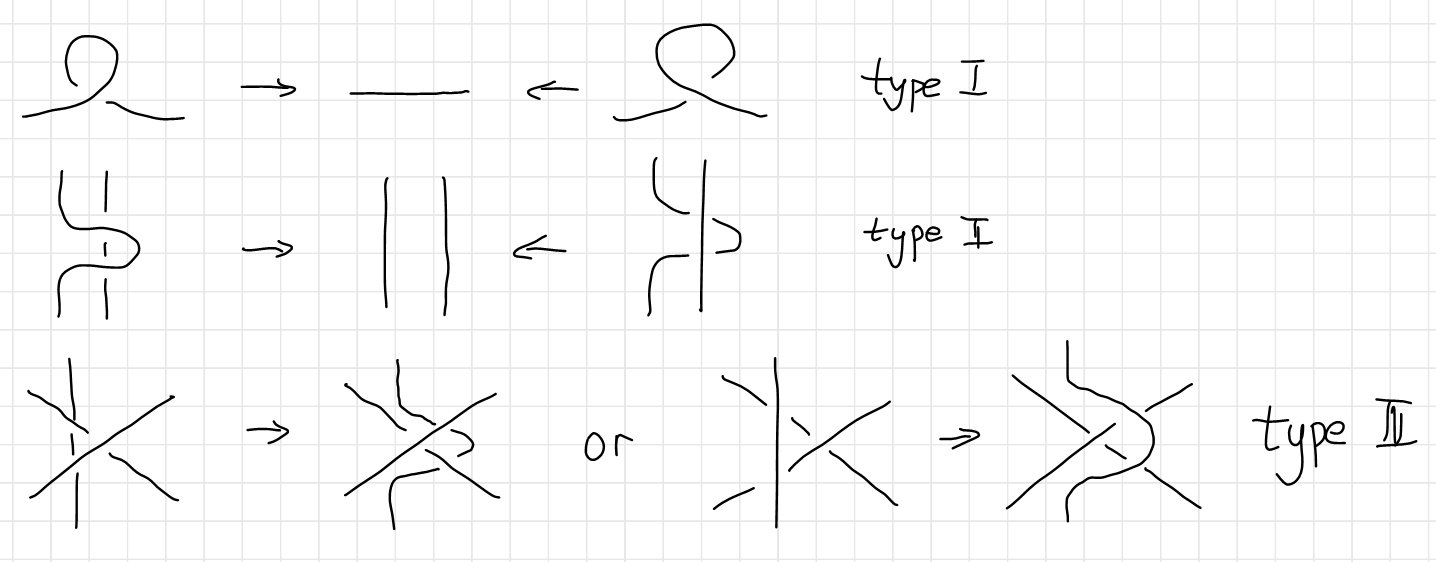
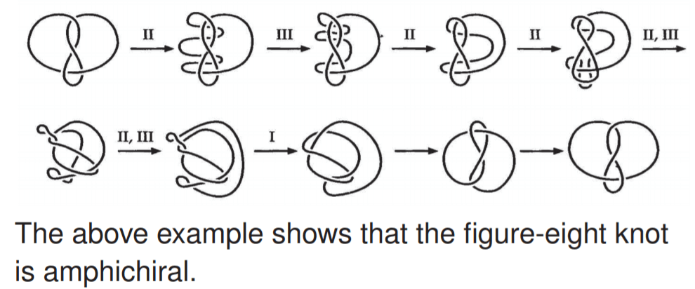
In 1920s, Reidemeister started to take a more formal path to tackle the problem of classifying the knots. He came up with the Reidemeister theorem ⁸ as a natural abstraction of “untying the knots”, stating that two knots are topologically equivalent if and only if their projections may be deformed into each other by a sequence of the three moves shown below.

This theorem is the foundation of all knot theory. It has become the touchstone for all knot invariants, and has been the philosopher’s stone in the conception of many knot invariants. Here is an example of two knots undergoing the Reidemeister moves (Image source).

Although the Reidemeister theorem is a huge success in telling us how to deform a knot step by step, the theorem itself contains no information of how to simplify a certain knot. Making matters worse, given a diagram of an unknot to be unknotted, it might be necessary to make the diagram more complicated before it can be simplified. We call such a diagram a hard unknot diagram. A nice example of this is the Culprit. If you look closely, you’ll find that no simplifying type I or type II Reidemeister moves and no type III moves are available.⁹

A natural question arises: “Is the trefoil knotted at all?” Since we cannot exhaust the infinite moves on a knot, we are unable to make the conclusion that the trefoil is knotted simply because we can’t find a series of Reidemeister moves. For all we know, there might be a way to deform a trefoil to a unknot, we just didn’t know yet. Of course a trefoil is knotted, the question is how to prove it. To prove trefoil is knotted, mathematicians came up with a knot invariant called the tri-colorability.

Intuitive Knot Invariants: Tri-colorability

The most intuitive knot invariant is tri-colorability ², which maps knots into the set $\set{\text{True}, \text{False}}$.

A knot (or a link) is tri-colorable if each strand can be colored in one of three colors with the following rules:

1. At least two colors are used.
2. At each crossing, either all three colors are present or only one color is present.

Here are tricolorings of a few knots (Examples source 1, Example source 2).

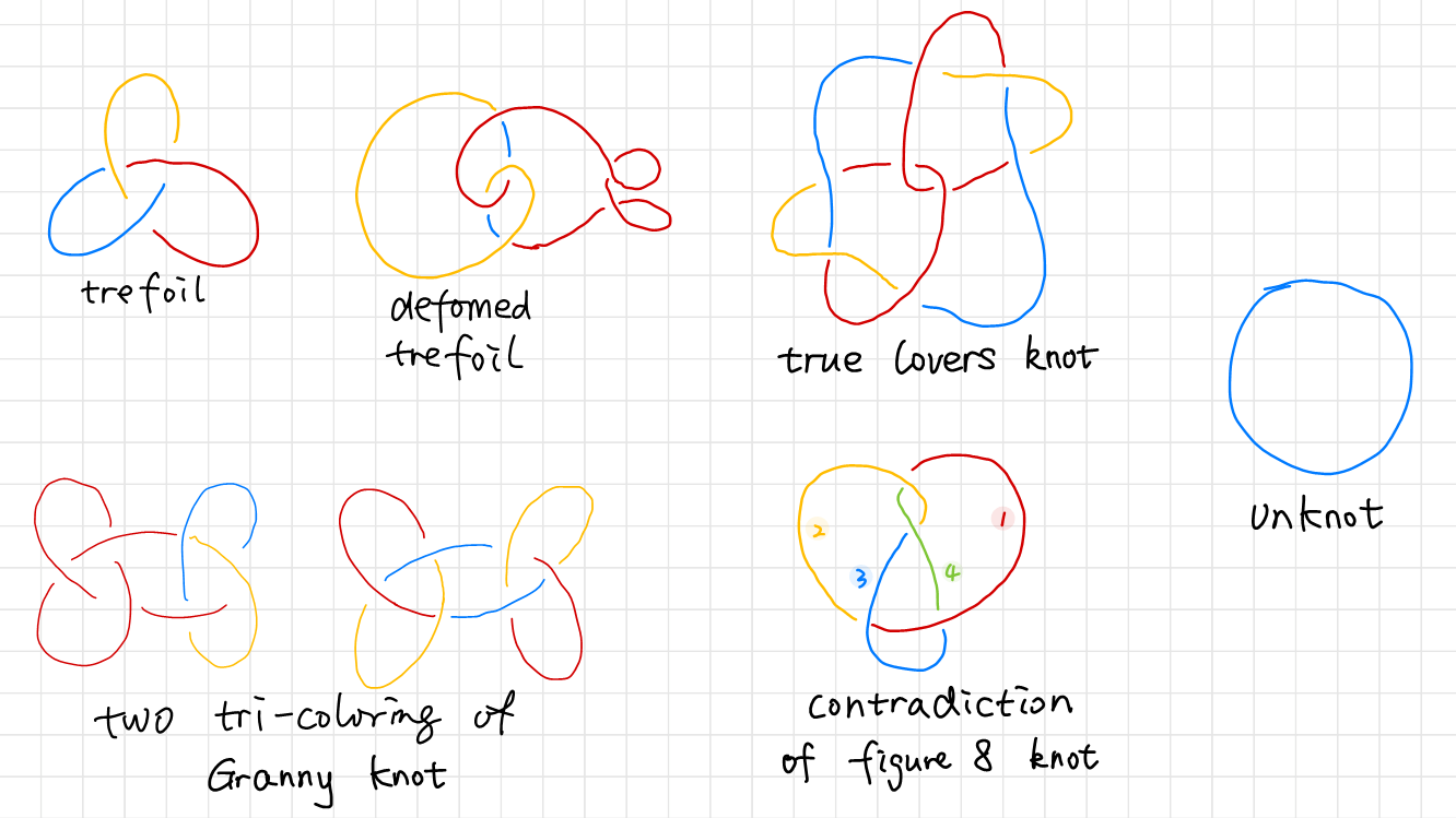
You can try it yourself, but you can never tri-color a figure eight knot. It can be shown that all four strings labeled from $1$ to $4 $ need to be in different colors. Although it might not be easy to show that all tri-colorings of some other knot is illegal, it’s very easy to show that the unknot is not tri-colorable, while the trefoil is tri-colorable. We found from deforming the tricolored trefoil that tri-colorability is unaffected by a deformation. If we can show that tri-colorability is a knot invariant, we will be able to prove that there are at least two types of knots, one of them is tri-colorable, the other is not. The unknot and the trefoil belongs to different types.

Proof of Tri-colorability Is a Knot Invariant

To prove that tri-colorability is a Knot Invariant, all we need to do is to prove that tri-colorability is unaffected by the three Reidemeister’s moves.

The first Reidemeister’s move is the straightening of a twisted string. Since the twisted string self-intersecting, it can only be in one color.

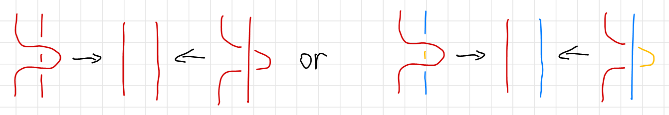
The second Reidemeister’s move’s tri-coloring has two cases drawn below. Either the two strings are of the same color, which is the trivial case, or the two strings contains all three colors.

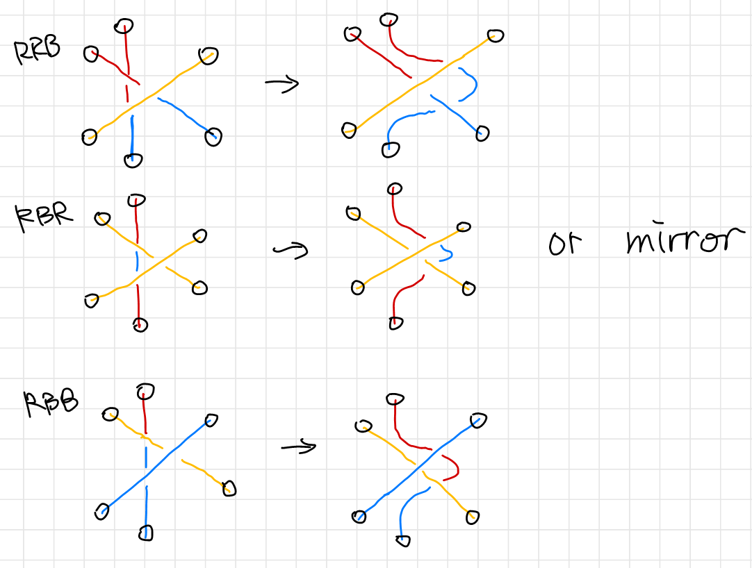
The third Reidemeister’s move’s tri-coloring has three nontrivial cases as is shown below. The trivial case is omitted since all three stings has the same color. The cases are classified by the color ordering of the vertical string as is indicated on the right of each case. Notice that colors at end of each string (circled in black) is un changed. The second scenario of the third Reidemeister’s move is merely a $60^\circ$ rotation of the first scenario.

Thus we have proven that the three Reidemeister’s move preserves tri-colorability. In other words, tri-colorability is not affected by continuous deformations or “un-tying of the knots”, and hence a knot invariant.

Consequences of Tri-colorability

Since a trefoil can be tri-colored and a unknot can’t, and tricolorability being a knot invariant, we have proven that the trefoil is indeed knotted. Which is the perfect example of how mathematicians go out of their ways to prove things that does not require proving. However, such tri-colorability can be generalized to $N$-colorability.

Algebraic Knot Invariants

Remember the figure eight knot. It cannot be tri-colored, but can be quad-colored. Is quad-colorability a knot invariant? (Interestingly, the figure eight knot is actually penta-colorable, see Figure Eight Knot is Penta-Colorable) It is also natural to ask if $N$-colorability is a knot invariant. To study $N$-colorability, clearly we cannot rely on drawing colorful diagrams of knots. For we will soon run out of distinguishable colors, and even coloring Reidemeister’s moves will become impossible.

Instead of colors we will use labels such as $1,2,3,\cdots$ on the diagram and replace the coloring rule by a method for combining these labels. Let’s see can we deduce from the tri-coloring scheme. For now we will use $a,b,c,\cdots$ to represent these colors.

Tri-coloring Revisited

We use $\set{1,2,3}$ to denote three colors. Recall the definition of tri-colorability:

A knot (or a link) is tri-colorable if each strand can be colored in one of three colors with the following rules:

1. At least two colors are used.
2. At each crossing, either all three colors are present or only one color is present.

We can translate the first requirement as there are at least two distinct elements in the set $\set{a,b,c}$. The second requirement can be translated as

\[\begin{array}{c} a\times a=a, \quad \text{only one color is present} \newline \text{or}\\ a\times b=c, \quad \text{all three colors are present}\newline \end{array},\quad \forall a,b,c \in \set{1,2,3}\]

where $\times$ is read as “cross”, as the string of color $a$ crosses string of color $b$.

A careful inspection on the following diagram reveals that we need to make a further distinction between an over-crossing and an under-crossing, since the two $a\times b$ are in different colors and cannot be the same, as is illustrated below.

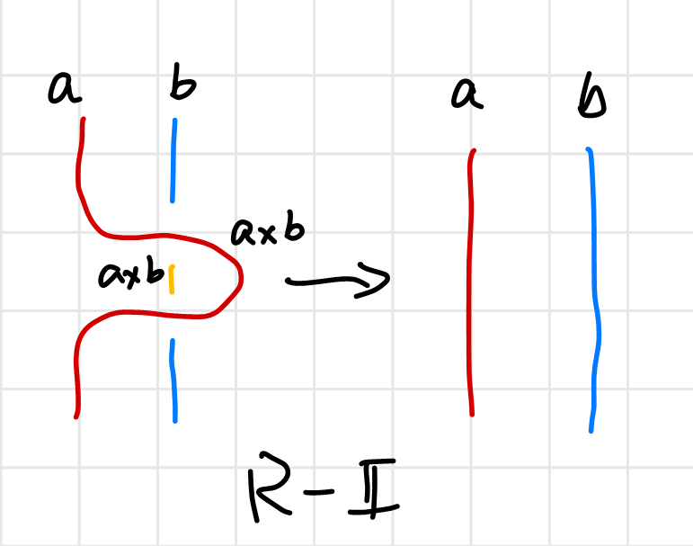
Also to spare ourselves from writing redundant equations as “$a$ goes over $b$ does not change color” such as $a\times_{\text{over}} b=a$, we will only make distinction between a left-handed or a right-handed crossing, and leave the upper string unchanged.

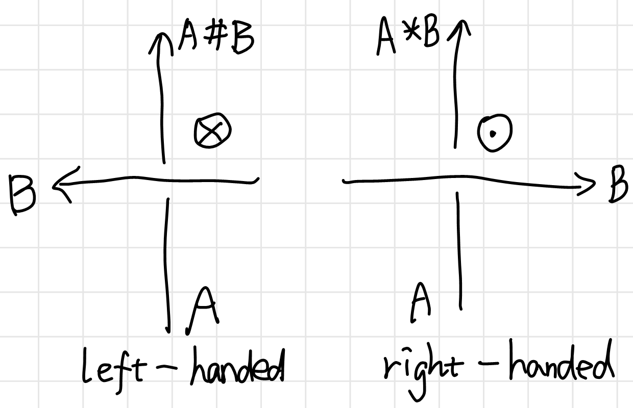
We assign to each string in a knot an arrow in a self-consistent way. If the cross product of the directional vector of the upper string and that lower string is outward-perpendicular to the page, we call the crossing right-handed, otherwise it’s left-handed. Or you can orient the lower string upward and the direction of the upper string determines it’s handedness. We use $a∗b$ to denote that string $a$ is right-handed crossed by $b$; and $a\hashtag b$ to denoted the other case as in ¹.

We can test out our labeling system in tri-color examples. All the crossing of the trefoil shown below are left-handed, hence

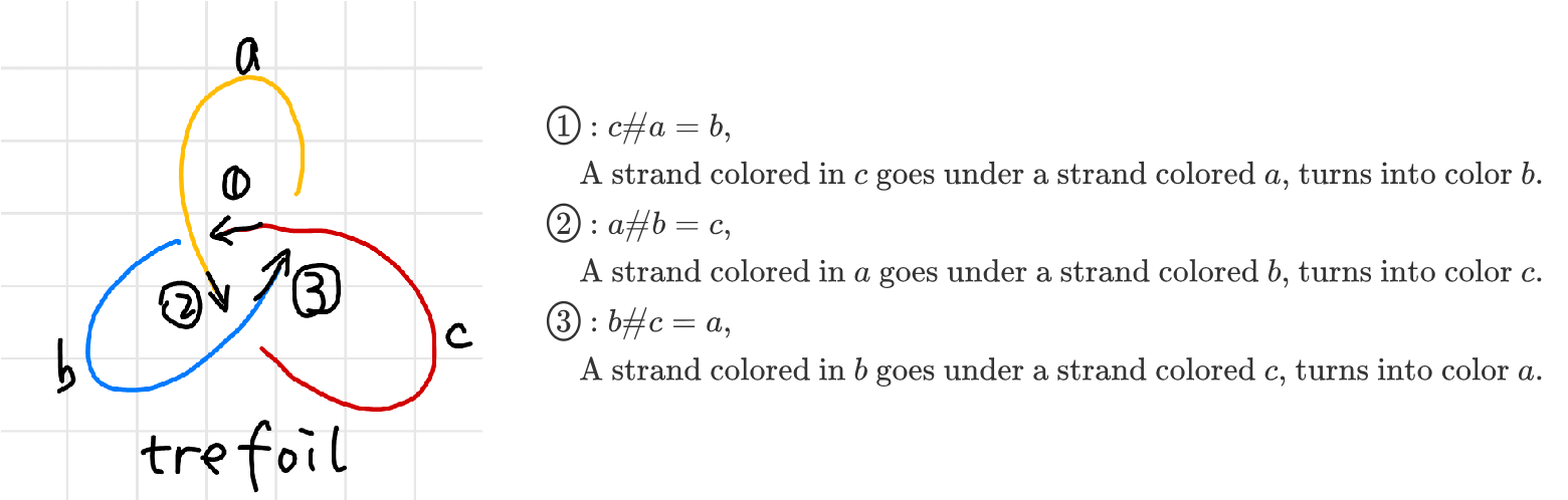
A further look at the trefoil soon reveals that $\hashtag $ is not associative. The same is true for $*$.

\[a\hashtag (c\hashtag b) = a\hashtag a = a \\ (a\hashtag c)\hashtag b = b\hashtag b = b\]

Now let’s translate the color rules to label rules using the Reidemeister’s Theorem.

Obtain the $N$-coloring Rules

In this section, we are using $N$ colors (labels), denoted as $\set{a,b,c,d,\cdots}$. Although there are only $26$ letters, we imagine that we will never run out of characters, also because $a,b,c$ is always nicer to read than $a_1,a_2,a_3$. To avoid loss of generality, $a\hashtag b $ is left un-evaluated as a “color” as a whole.

The first Reidemeister’s move is evident.

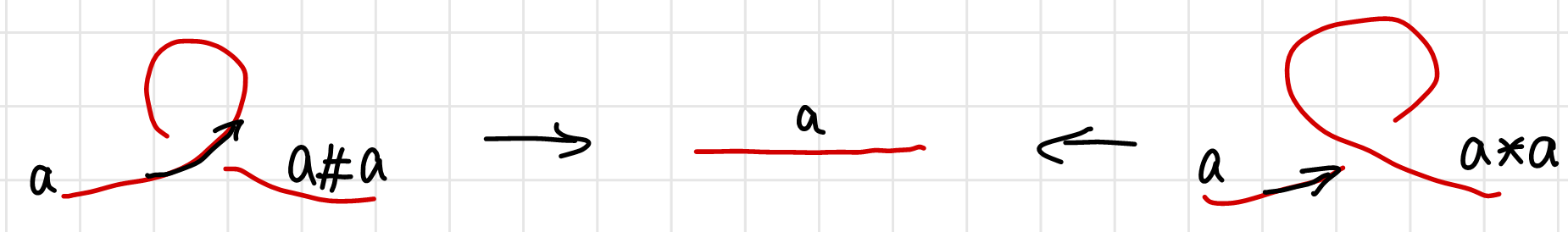
We have

\[a\hashtag a =a , \quad a* a = a\]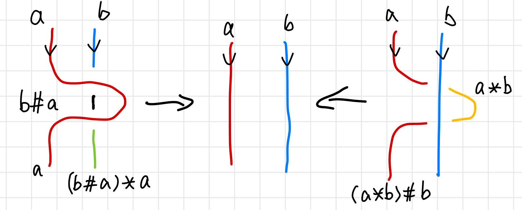

---

The second Reidemeister’s move is a little complicated. I used more than three colors to color code it to avoid confusion (since $b\hashtag a\neq a*b$). The Reidemeister’s theorem requires that the corresponding ends have the same color.

\[(b\hashtag a)*a = b \\ (a*b)\hashtag b = a\]

From these equations, $\hashtag $ and $*$ looks like inverse operations to each other, which is discussed in detail in Chapter 3 in ¹⁰.

---

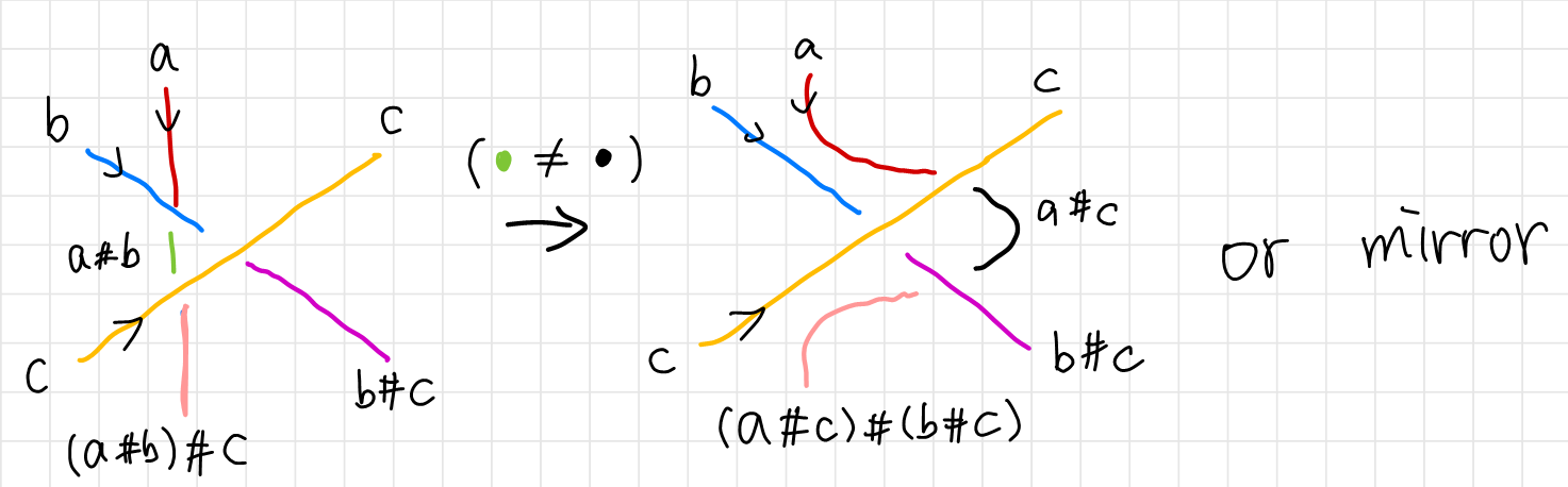
In the same manner we can get results form the third Reidemeister’s move. We require again that corresponding ends have the same color. The arrows on the diagram were carefully chose to obtain

From the above diagram, we have

\[(a\hashtag b)\hashtag c = (a\hashtag c)\hashtag (b\hashtag c)\]

and the mirror diagram would give the equation

\[(a*b)*c = (a*c)*(b*c)\]

---

Summarizing, we have an algebraic system satisfying these rules (correspond to three Reidemeister’s moves respectively):

1. $a*a=a$ and $a\hashtag a=a$ for any $a$
2. $(a * b)\hashtag b = a$ and $(a\hashtag b) * b = a$ for any labels $a$ and $b$.
3. $(a * b) * c = (a * c) * (b * c)$ and $(a\hashtag b)\hashtag c = (a\hashtag c)\hashtag (b\hashtag c)$ for any labels $a$, $b$, and $c$.

Color Rule as Modular System

A Linear Color Rule

The upshot is that we could use numbers $\set{1,2,3,\cdots,N}$ to represent $N$ different colors, and feed these numbers in the law of $*$ and $\hashtag $, and find out the coloring relations between them. Let’s suppose that these two operations are liner, that is

\[\begin{align*} a * b &= x^* a + y^* b\\ a \hashtag b &= x^\hashtag a+y^\hashtag b \end{align*}\]

Using the three laws it’s easy to find out that

\[\begin{array}{crlrl} \text{law 1: } & x^* +y^* =1, &x^\hashtag +y^\hashtag = 1\\ \text{law 2: } & x^*x^\hashtag =1, &x^\hashtag x ^* = 1\\ \text{law 3: } & \begin{cases}x^*y^*=y^*x^* \\ y^*(x^*+y^*-1)=0 \end{cases} , &\begin{cases}x^\hashtag y^\hashtag =y^\hashtag x^\hashtag \\ y^\hashtag (x^\hashtag +y^\hashtag -1)=0 \end{cases}\\ \end{array}\]

Starting from the law 3. If $y^ * =0$ or $y^\hashtag =0$, then we could only use one color since $a * b=a\hashtag b = a$, $\forall a\in \set{1,2,\cdots,N}$. Hence the non-trivial linear color rule would be

\[a * b =t a + (1-t) b \\ a \hashtag b = \tfrac{1}{t} a+(1- \tfrac{1}{t}) b\]

Note that strangely law 3 does not provide much useful information, I think it’s partly due to our color law is linear.

Why a Linear Color Rule Is Incorrect

To give an example of the aforementioned linear color rule, consider a special kind of color rule such that $a ∗ b = a\hashtag b$, namely set $t=1$. We have

\[a * b = a\hashtag b = 2b-a\]

Put the law into the relationships we obtained in Tri-coloring Revisited, we have

\[a*b =2a-b = c\\ b*c =2b-c = a\\ c*a= 2c-a = b \label{tri-color-modul}\]

The above equations lead disastrously to $a=b=c$. This means that our linear system simply does not work. Which should have been obvious in the last chapter, but is more evident only after we are working with actual numbers. If we pick a set of values for $a$ $b$ and $c$, we would run into the problem as below.

\[\begin{array}{rccccr} &\color{red}\text{red} & crossing &\color{blue}\text{blue} & gets & \color{orange}\text{orange} \\ \text{instead of :}&1&*&2&=&3\\ \text{we have :}&1&*&2&=&2\times 1-1=0 \\ \end{array} \\ \begin{array}{rccccr} & \color{orange}\text{orange} & crossing &\color{blue}\text{blue} & gets & \color{red}\text{red}\\ \text{instead of :}&3&*&2&=&1\\ \text{we have :}&3&*&2&=&2\times 3-2 = 4 \end{array}\]

It’s obvious that the discrepancy gets worse if we keep going. Color $\color{red}\text{red}$ would go from $1$ to $4$ to $7$ …, and $\color{orange}\text{orange}$ from $3$ to $0$ to $-3$… Eventually we will go to $\pm \infty$ if we keep updating the numbers.

Modular System on Tri-colorability

The minimal modification we can make to a linear color rule is making it a modular system. We want $1,4,7,\cdots$ to represent the same color, $3,0,-3,\cdots$ to represent another one. The obvious solution is take the module of $3 $ for $a$, $b$ and $c$.

In other words, we represent colors using $\ints/3\ints=\set{1,2,3}$ to represent the numbers, and modify the rules to be

\[a * b = a\hashtag b = (2b-a)\mod 3\]

which is hinted by $\Eqn{tri-color-modul}$, if we sum all of the equations we will have $3(a+b+c)=0$.

Figure Eight Knot is Penta-Colorable

As a side note, although you can color the figure eight knot using merely four colors, the algebra requires a modulo system of $5$. This can be shown as follows: pick the two string highlighted in red and set them to be $a$ and $b$. Work around the knot and meet at the string highlighted in green. We have $5(a-b)\equiv0$, which means $a=b$ (trivial coloring) or it’s a modular $5$ coloring.

The same technique can be applied to other knots, as is show on the right. $7(a-b)=0$ means that the knot to the right is $7$ colorable, though there are only $5$ strands.

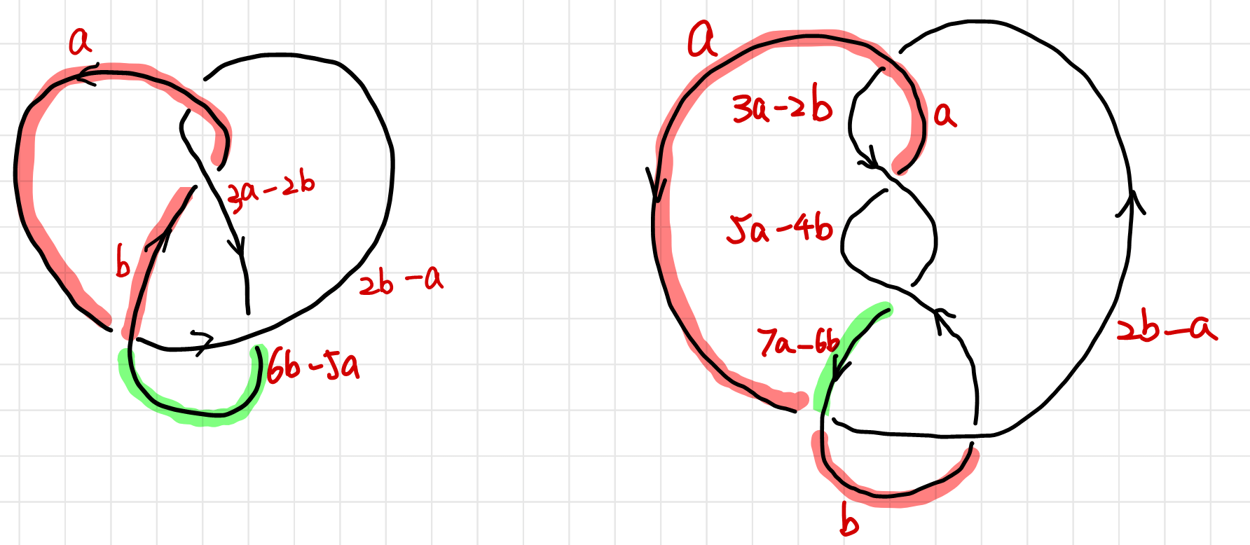
The above examples shows that our coloring rule “At least two colors are used” should be modified according to $N$. In the following discussion, we will simple require “More than one color is used”.

Polynomials as Knot Invariants

Coloring Equations and Coloring Matrices

This section follows ¹¹.

Coloring Equations of a Knot

So far we have worked out the coloring relations, namely how to device an algebraic rule on the ring $\ints/N\ints$. So far we only discussed the coloring for the trefoil, which is actually done by “trial and err”: We assign an arbitrary color to an arbitrary strand and work our way to the next. We assume the next strand may have a different color and see if there is an contradiction. Luckily there is none for trefoil. But we cannot say that for any knot, especially when the knot are complicated. In this section we will consider $a\hashtag b = a*b = 2b-a$ unless otherwise stated.

To find all possible colorings of a knot, we will have to turn the problem into a solution of a set of equations. We will define -coloring as a map from strands of a knot to the a set of integers, $\set{1,2,3,\cdots,N}$. If we label the strands as $\set{x_1,x_2,\cdots,x_m}$, the map can be written as: $\chi: \set{x_1,x_2,\cdots,x_m} \rightarrow\set{1,2,3,\cdots,N}$. We will have $m$ equations at $m$ crossings (if there is no closed loop in the knot, as is shown below, the red string is a closed loop and can be removed),

and each solution of $\set{x_1,x_2,\cdots,x_m}$ is a valid coloring. For example, the trefoil and the figure eight knot has the following coloring equations:

\[\begin{array}{rrrrrrr} \alpha:& 2 x_1& - x_2& - x_3 &= 0 \mod N\\ \beta :& - x_1& +2 x_2& - x_3 &= 0 \mod N\\ \gamma:& - x_1& - x_2& 2 x_3 &= 0 \mod N\\\\ \end{array} \qquad\qquad \begin{array}{rrrrrrr} \alpha:& 2x_1 & - x_2 & & - x_4 &= 0 \mod N\\ \beta :& & 2 x_2 & - x_3 & - x_4 &= 0 \mod N\\ \gamma:& -x_1 & - x_2 & +2 x_3 & &= 0 \mod N\\ \delta:& -x_1 & & - x_3 & +2 x_4 &= 0 \mod N\\ \end{array}\]

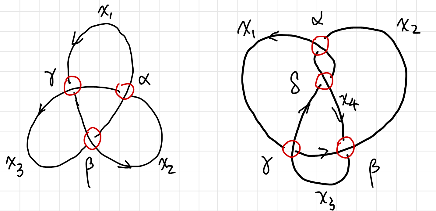
These equation is linear equations defined on a modular system, which is not very different from common linear equations. Obviously the trivial coloring $x_i=0$ (or equivalently $x_i=N$) is always a solution.

Properties of Coloring Equations

Notice that the coloring equations are not all independent. Since all the equations sum to zero. Also if $\set{x_1,x_2,\cdots,x_m}$ is a solution, so is $\set{x_1+k,x_2+k,\cdots,x_m+k}$. We can always set $x_m=N\equiv 0$ in the equation. Therefore we only need two variables and two equations for an non-trivial solution.

Thus the equation can be simplified as

\[\begin{array}{} M_\text{trefoil} \cdot (x_1,x_2,x_3)^T=0 &\rightarrow& \tilde{M}_\text{trefoil} \cdot (x_1,x_2)^T=0\\ M_\text{figure 8} \cdot (x_1,x_2,x_3,x_4)^T=0 &\rightarrow& \tilde{M}_\text{figure 8} \cdot (x_1,x_2,x_3)^T=0 \end{array}\]

where we take the upper left part of the original matrix

\[\begin{array}{} M_\text{trefoil} = \begin{pmatrix} 2 & -1&-1\\-1&2& -1 \\ -1 & -1 & 2\end{pmatrix} &\rightarrow & \tilde{M}_\text{trefoil} =\begin{pmatrix} 2 & -1\\-1&2\end{pmatrix}\\ M_\text{figure 8} = \begin{pmatrix} 2 & -1&0&-1\\0&2& -1&-1 \\ -1 & -1 & 2&0\\ -1&0&-1&2\end{pmatrix} &\rightarrow & \tilde{M}_\text{figure 8} =\begin{pmatrix} 2 & -1&0 \\0&2& -1 \\ -1 & -1 & 2\end{pmatrix} \end{array}\]

The matrix’s determinant is actually the number $\vert N\vert $ of $N$-colorability. $\det(\tilde{M} _ \text{trefoil})=3$, and $\det(\tilde{M} _ \text{figure 8} )= 5$ as is calculated before. The matrices $M$ are called the coloring matrix, $\tilde M$ the reduced coloring matrix.

Coloring Matrix as a Knot Characteristic

Why the coloring matrix’s determinant is related to a knot invariant? To answer this question, it’s better if we see it from J. W. Alexander’s perspective, who invented the famous Alexander’s polynomial. Here is my guess of how he came up with the idea.

A knot’s property is completely determined by it’s crossings. Once the types of each crossing, and how each crossing are connected are chosen, the knot is uniquely defined. If we can arrange the information of each crossing in some order, preferably in a table, we will establish a one-to-one correspondence between a knot diagram and a “table” which we can conveniently turn into a matrix. We might be able to gain some insight into how to extract an invariant from the diagram.

One candidate of such table is as below

	strand $1$	strand $2$	strand $3$	strand $4$	$\cdots$	strand$m$
crossing $1$	over-strand-to-left		strand-in	strand-out
crossing $2$		strand-out				over-strand-to-right
crossing $3$		strand-in
$\vdots$
crossing $m$				strand-in

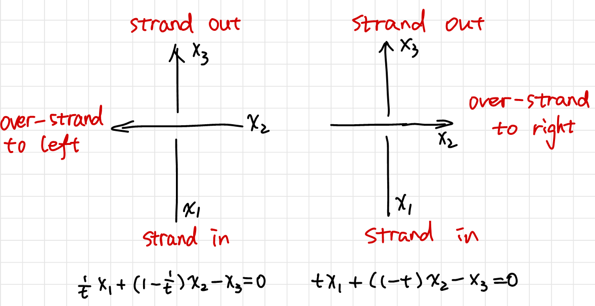
Conveniently, our linear color rule provide us with an algebraic way to represent each type of crossings.

\(\begin{cases} a * b =t a + (1-t) b \\ a \hashtag b = \tfrac{1}{t} a+(1- \tfrac{1}{t}) b \end{cases} \rightarrow \begin{cases} x_\text{out} =t x_\text{in} + (1-t) x_\text{over-left} \\ x_\text{out} = \tfrac{1}{t} x_\text{in}+(1- \tfrac{1}{t}) x_\text{over-right} \end{cases}\)

Thus the above table can be transferred to the following matrix

\[\begin{array}{cccccccc} &\text{strand $1$}&\text{strand $2$}&\text{strand $3$}&\text{strand $4$}&\cdots&\text{strand $m$}\\ \text{crossing $1$}\\ \text{crossing $2$}\\ \text{crossing $3$}\\ \vdots\\ \text{crossing $m$}\\ \end{array} \hspace{-12 cm}\matrix{\\ \quad1-t\qquad & \qquad&\quad t\qquad& \quad -1\quad& \quad& \qquad\\ \quad \qquad &-1\qquad&\quad \qquad& \quad \quad& \quad&(1-1/t)\qquad\\ \quad \qquad &1/t\qquad&\quad \qquad& \quad -1\quad& \quad& \qquad\\ \quad \qquad & \qquad&\quad \qquad& \quad \quad& \quad& \qquad\\ \quad \qquad & \qquad&\quad \qquad& \quad t\quad& \quad& \qquad\\ }\]

Thus the coloring matrix faithfully characterizes a knot diagram in that we can re-construct the knot diagram from the coloring matrix.

Alexander Polynomial from Coloring Matrix

If there is a knot invariant associated with the coloring matrix, it almost has to be the determinant. It involves all the entries (unlike the trace) hence it is “faithful”, and more importantly, it is invariant under unitary transformations. Our knot diagram can be seen as projection of a $3$-dimensional knot. Therefore different knot diagrams of the same knot is related to each other by a unitary transformation. (Although we do not consider deformation of the same knot as unitary transformation.)

Since the determinant of the coloring matrix is $0$, we will use reduced coloring matrix instead. The determinant of the reduced coloring matrix $\tilde M$ of a linear coloring rule is a Laurent polynomial of $t$ with integer coefficients. This polynomial is called the Alexander Polynomial, named after its discoverer J. W. Alexander.

Alexander found his polynomial in a similar way. He started off by a different way of forming the knot table, but arrived at the same conclusion. For an easy introduction, see ¹².

Many textbooks I have read either took an axiomatic approach as was introduced by Conway, or a very mathematical way all the way from fundamental groups, or “from the abelianization of $\ints [\pi_1 (\Reals^3/ K)]$”¹³. If you are interested, you can find out more in the Further Reading section.

The invariance of the determinant can be proven using Reidemeister’s moves, omitted here. Proof see ¹⁴.

Examples of Alexander Polynomials

We can calculate the Alexander polynomial using the coloring equations

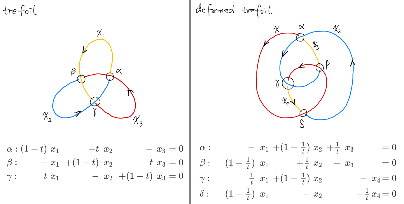\(M_\text{trefoil}=\pmatrix{1-t & t&-1\\ -1 &1-t&t\\ t & -1 & 1-t} \qquad M_\text{deformed trefoil}=\pmatrix{-1 & 1-\tfrac{1}{t}&\tfrac{1}{t}&\\ 1-\tfrac{1}{t} &\tfrac{1}{t}&-1&\\ \tfrac{1}{t} & 1-\tfrac{1}{t} & & -1 \\ 1-\tfrac{1}{t} &-1 && \tfrac{1}{t}}\)

And the Alexander polynomial for the above diagrams of the same knot are

\[\det(M_\text{trefoil}) =1-t+t^2 \\ \det(M_\text{deformed trefoil})=-1 - \tfrac{1}{t^2} + \tfrac{1}{t}=-t^{-2}(1 - t + t^2)\]

Note that they differ by a factor of $-t^{-2}$. Alexander polynomial is still a modular system, such that polynomials differ by a factor of $\pm t^{n}$ are the same in a “modular sense”. To show that Alexander polynomial is indeed a knot invariant that sets different types of knots apart, here is the figure eight knot,

\[\begin{array}{rrrrrrr} \alpha:& (1-t)x_1 & +t x_2 & x_3 & &= 0\\ \beta :& -x_1 & & +(1-t) x_3 & &= 0 \\ \gamma:& \tfrac{1}{t}x_1 & - x_2 & & +(1-\tfrac{1}{t})x_4 &= 0 \\ \delta:& & +(1-\tfrac{1}{t})x_2 & +\tfrac{1}{t} x_3 & -x_4 &= 0 \\ \end{array}\]

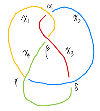
and its Alexander polynomial is different from that of trefoil.

\[\det(\tilde M_\text{figure eight})=1 - 3 t + t^2\]

Skein Relations

Alexander found out in his paper that the Alexander polynomial of “similar knots” have certain relations, which he then listed in a chapter titled “Miscellaneous theorems”.

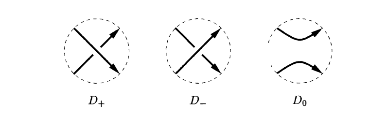
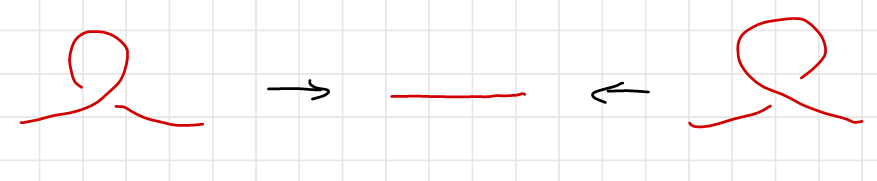
If three oriented links $L _ -$, $L _ +$ and $L_0$ have diagrams $D _ -$, $D _ +$ and $D_0$ which differ only in a small neighborhood as shown above, then \(\Delta(L_+)-\Delta(L_-)=(x^{-1}-x)\Delta(L_0)\) Conway (whose name you could have heard from the game of life) rediscovered and reformulated it as a set of recursive rules called the “skein relations” 30 years later ⁷.

Conway’s idea was “to consider knot invariants not as maps of the set of knots to the set of polynomials (for instance), but as maps from some sort of space of knots, locally characterized by how they behave on knots in ‘close proximity’. “¹⁵

The significance of the skein relation is that it allows us to abandon the tedious calculations of the coloring matrix, and turn the algorithm for obtaining the Alexander polynomial into a child’s play.

An example would be as below.

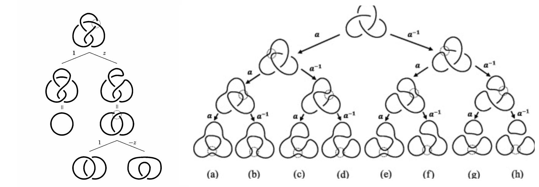
For a long time why such skein relations would work remained a mystery. Turns out the skein relation is deeply connected to various fields in physics, such as statistical mechanics and quantum field theory, which we shall discuss in the following section.

Jones Polynomial and Beyond Knots and Physics

Discovery of Jones Polynomial and Its Influence

In the summer of 1982, Vaughan Jones was presenting a lecture on von Neumann algebras in Geneva. At the end of his talk Didier Hatt-Arnold, a graduate student in the audience, suggested that the relations in his algebraic structures were similar to those in the braid groups. Soon afterwards, Jones worked out how to construct representations of the braid groups into his algebras, but he did not immediately recognize their significance. The following summer, Jones realized that the image of $\mathbb B _ 5$ under one of the representations was the projective symplectic group $\mathrm{PSp}(4, \ints _ 3)$, the finite simple group of order $25920$. Thinking that this might be of some interest, Jones arranged to discuss his representations with Joan Birman.

Jones travelled to New York in May 1984. He and Birman soon showed that this was not just another technique for deriving the Alexander polynomial. One simple test proved that this invariant was new: it could distinguish the left-handed and right-handed trefoils! Jones later established that his polynomial also satisfies a skein relation: ¹⁶

\(tV(L_+) - t^{-1}V(L _ -) = (t^{1/2}-t^{-1/2})V(L_ 0 )\) This discovery had a tremendous impact, and not only on knot theory. Once it was known that the Alexander polynomial was not the only polynomial link invariant, people started to search for more, some using combinatorics and others following the algebraic route used by Jones. Close connections with physics generated a lot of interdisciplinary research, and polynomials were defined via physical methods related to statistical mechanics, where the Yang-Baxter equation provides an analogue of the third braid relation, and quantum groups. These new link invariants were also extended to give invariants of 3-manifolds.

What we need to know now is that this was a highly complicated history and a somewhat “accidental” discovery. However, such polynomial can be found by defining a new set of skein relations. This new type skein relation fueled the search for more polynomials by choosing different skein relations. Later the HOMFLY polynomial were quick discovered by choosing yet another skein relation.

However, such skein relation remained largely as a mathematical trick for calculating the corresponding polynomials, without knowing “why this would work”. Later Witten realized that the Jones polynomial is related to QFT, as according to the path integral formalism, particles may travel freely forward and backwards in time. Thus a particle confined in $2$-dimensional space can have a “knotted” trajectory in $(2+1)$ space-time. The knottedness is related to Chern-Simons theory and it turns out that the amplitude of a trajectory is related to whether the trajectory is knotted or not. This point of view gave birth to the Kauffman bracket, which we should discuss in detail below. For more information, you can read [^Ap-physics] and ¹⁷. For the original definition, see chapter 4 of ¹⁸.

Polynomials and Physics

I spent quite some time trying to sort out the logic between these polynomials for about a month, decided to give it a rest, and gave it another week after a 2 months break. I have to say regrettably that I have not seen a introductory paper or book that dumbed down the relations of polynomials and physics to a level that I could understand.

Apparently there are two kinds of connections, one is with statistical mechanics, which we start from arranging knots on an Ising model. (See 2. Spin models, the Potts model, IRF models of ¹⁹ or ¹⁶.) The other is with quantum field theory or an enhanced version of it (topological QFT etc.), where a expectation value is assigned to the vacuum. (See Chapter 8. Knot Amplitudes of ¹ .)

What I struggle with is that I could not answer why such arrangements were made. They seemed to me as a effort to force the idea of knot theory on a physical system. I don’t have the knowledge needed to understand it comprehensively so I have to end it here. If you have any suggestions or any directions you can provide me to chase, feel free to leave a comment. This crash course has gone way out of my expectation so far and I might circle back if I need more knowledge on knot theory.

Further Readings

Time-line of history: Collberg, E. (2017). A brief history of knot theory. Página consultada a, 8.

Daniel Moskovich, How to motivate the skein relations?, URL (version: 2010-04-06): https://mathoverflow.net/q/20505

Fun tricks with knots. Plus a history Kauffman’s lecture at KITP: Revolutions in Knots, Braids and Physics, Louis Kauffman.

NJ’s brief history of knots: <https://www.youtube.com/watch?v=KYddgeiyLJ8

YouTube Video Tying Things Together: Knots in Maths, Physics and Biology’ - Dr David Skinner. factorizing and knot: jones polynomial similarity: 21:36

Witten’s talk https://www.youtube.com/watch?v=cuJY14BYac4

Knot theory and CHern simons, probably not very useful later. https://www.youtube.com/watch?v=8wWvUJ6qJx0

Jones’s intro to Jones Polynomials. https://math.berkeley.edu/~vfr/jones.pdf Jones, V. F. (2005). The Jones polynomial. Discrete Math, 294, 275-277.

A very mathematical way of introducing the tri-colorability as quandles, keis, etc. : Quandles: An Introduction to the Algebra of Knots

Knots and “universe” Kauffman, L. H. (2006). Formal knot theory. Courier Corporation.

Nice intro but lacks explanation of Jones: ²

Knots on a Torus Kauffman, L. H. (1998). Virtual knot theory. arXiv preprint math/9811028.http://homepages.math.uic.edu/~kauffman/VKT.pdf

Might be important when calculating braiding on PBC

---