---

\[\newcommand{\ket}[1]{\vert {#1} \rangle} \newcommand{\bra}[1]{\langle {#1} \vert} \newcommand{\braket}[2]{\left\langle {#1}\! \mid \!{#2} \right\rangle} \newcommand{\Partial}[2]{\frac{\partial {#1}}{\partial{#2}}} \newcommand{\emath}{\mathrm e} \newcommand{\R}{\mathbb R}\]

This post mainly follows Nakahara.

Motivations

I might have stated this in a few other notes but I will state here again. There are many topological invariants that give different insights to the property of a manifold. One of the most famous topological invariants is probably the genus which is a number usually associated with holes of the surface. A student in the field of condensed matter physics probably has heard the Chern number.

But a topological invariant can also be an algebraic entity instead of a number, such as a group. If we associate a manifold a group and the group is invariant against local deformations, we can call this group a topological invariant as well.

We can imagine that saying a group as a topological invariant of a manifold is going to reveal far more properties than just a number. That’s what we are going to do in this post.

Path and Loops

Circles and Holes

We have already encountered the genus which is closely related to the number of holes of a surface. To find a genus of a surface we can first triangulate it and calculate the Euler’s number of the surface. Or by

==[????what was the cohomology group doing? I forgot]==

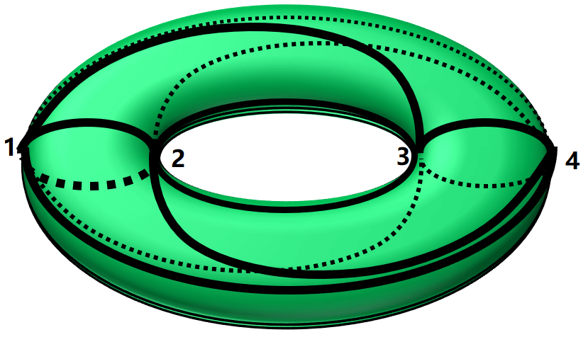
There is another way to detect holes of a surface. To do that, look at the torus below.

There are at least three types of circles on the surface. By types we mean topologically inequivalent, i.e., cannot deform into each other. We can deform the red one and shrink it as much as we want and eventually we can shrink it to a point. So the red circle is topologically equivalent to a point whereas the blue circle does not. You cannot shrink the blue circle anymore. So is the yellow one. Moreover, you cannot deform the blue circle to the yellow one. So there are at least three types of circles on the surface of a torus.

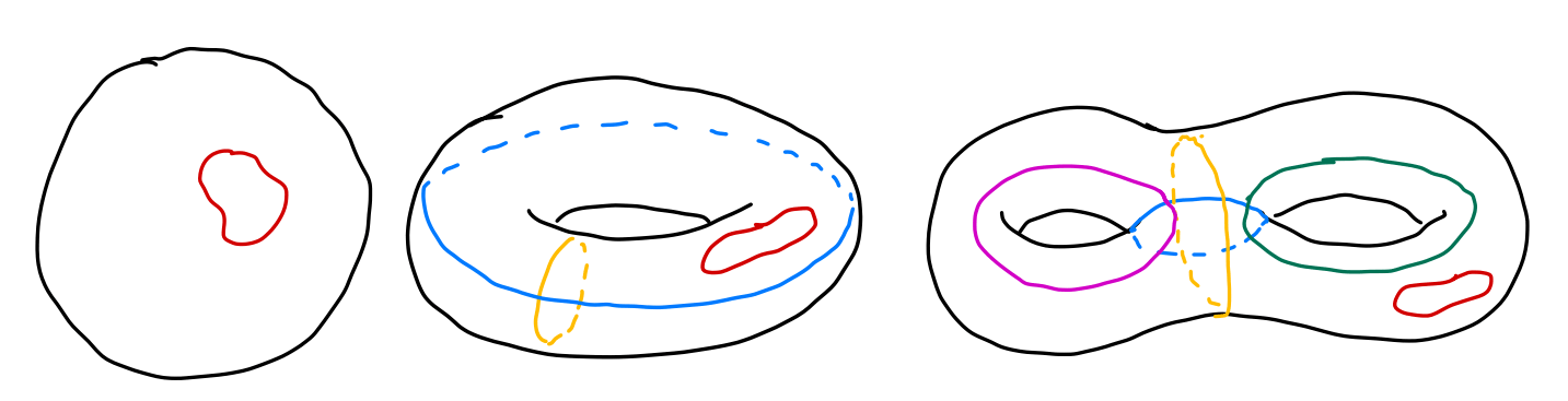
On the other hand, all circles on a sphere are contractible, meaning they are all topologically equivalent to a point. Circles on a two-holed torus are more complicated but the results are shown above as well.

Obviously, the above results are topological, as we can deform the manifold continuously but the conclusion remains the same. So in some sense, the number of inequivalent circles can be used as a topological invariant. Mathematically it’s hard to prove that “there is no way to deform the circles into one another”, or to prove “there are only these types of circles on the surface”. To do that, we are going to use some definitions.

If you are not interested in the mathematical details, you can jump directly to Calculation of Fundamental Groups

Mathematical Structures among Paths and Loops

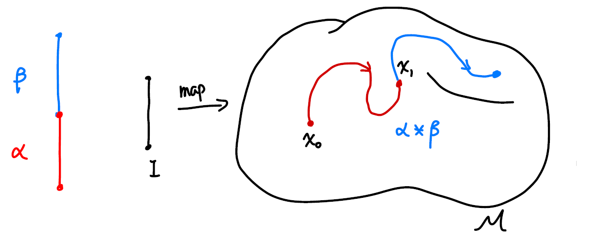
A path on a manifold can be seen as a map from an interval in real axis $I=[0,1]\in\R^1$ to a (continuous) line on the manifold $\mathcal M$. We denote the map as

\[\alpha: I\rightarrow \mathcal M,\]

where $\alpha(0)=x _ 0$ and $\alpha(1)=x _ 1$ are considered the beginning and the end of the line. We will from now on use the map $\alpha$ to indicate the path on the manifold.

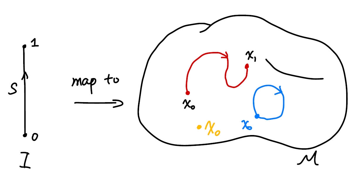
If $x _ 0=x _ 1$, naturally we call $\alpha$ a loop that start at $x _ 0$ or whose base point is $x _ 0$.

What’s interesting about the path and circles defined about is paths as a set behave like a group.

First, we can define a multiplication between a path $\alpha$ and a path $\beta$ as $\alpha * \beta$, where

\[\alpha * \beta(s) = \cases{ \alpha(2s),\quad 0\le s \le 1/2\\ \beta(2s-1),\quad 1/2\le s \le 1 }\]

Intuitively the operation is defined as moving along the first path and continuously transit to another with equal time spent on either of the paths. Hence we require that for our multiplication to give a continuous path, the second path must start where the first path ends.

Note that the coefficients in the map can be defined in other ways as well, say

\[\alpha * \beta(s) = \cases{ \alpha(8s^2),\quad 0\le s \le 1/8\\ \beta((8s-1)/7),\quad 1/8\le s \le 1 }\]

is the same path on the manifold. We made our choice but you can make yours. From now on we will use the former one for its simplicity.

The multiplication is associative, which we will prove later in this post. But we can see direct by manipulating the paths.

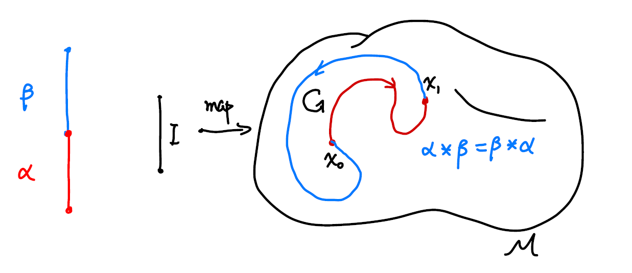
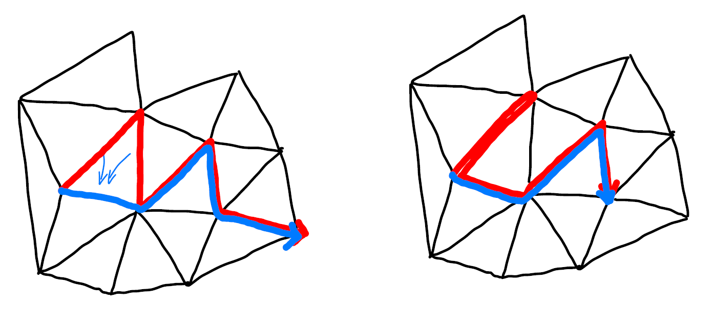
The multiplication is communitive, as the multiplication is defined in such a way that if $\alpha\beta$ and $\beta\alpha$ both exist, they must form a loop. The result of the multiplication is only going to be the same loop. As is indicated in the sketch below. The direction of the loop is indicated by the black arrow. There is a small nuance that even the results “overlap”, they actually give us “two loops with different base points”. We will address this issue later when we talk about homotopic maps.

The identity we choose here is going to be a constant map $c$ which correspond to a point in the manifold,

\[c _ {x _ 0} : I \rightarrow x _ 0\in \mathcal M\]

Obviously, the identity here is not unique and we will address that in a minute.

The inverse of a path is defined as traveling along the path reversely. The inverse is denoted as $\alpha^{-1}$,

\[\alpha^{-1}(s) =\alpha(1-s), s\in I\]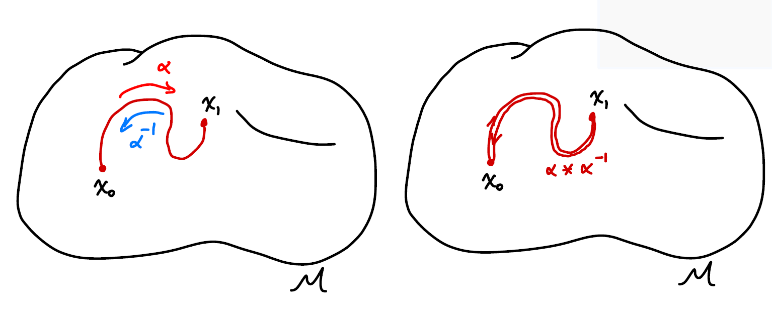

When a path is multiplied with its inverse it does NOT gives us the identity,

\[\alpha * \alpha^{-1}(s) = \cases{ \alpha(2s),\quad 0\le s \le 1/2\\ \alpha^{-1}(2s-1),\quad 1/2\le s \le 1 }\]

as traveling back along a path does not erase the path at all. Instead, we have a “double thread” or a collapsed loop.

And now all that’s left is closure. We can see that the results of the above operations are still paths. So we have an algebraic structure among the paths.

The operations defined above can be a bit awkward, as the inverse and identity’s definition does not fully match, and the multiplication only between the elements that have a least one common end. Things do look better if we look at only loops that start from a certain point. That way the multiplication does make more sense, but the inverse is still odd.

Making a Group

As is stated before, paths do not form a group under operations defined above. As definitions related to an identity in a group is that

Identity $e$ is the unique element from group $G$ such that for all $g\in G$,

\[eg=ge=g, \\ gg^{-1} = e.\]

Luckily, mathematicians know what to do with this type of situation. To make the set of loops with the aforementioned operations a group, we can treat a few elements as the same element, as dividing the elements into different classes. And if we do that in a clever way for other elements in the set as well and look at the multiplication between classes, we might be able to define a group.

Mathematically the “classes” are called equivalence classes, defined by equivalence relations

From the topology point of view, this “division by class” is natural as we do not care about the actual shape of loops, but their topology. We can continuously deform them on the manifold as much as we want but this will not alter the topological property of the paths. So we might as well pick one path from each “topological type” and study them.

Homotopy Relation Represented by $F$

Mathematically, we state the equivalence relation defined as homotopic relation:

Let $\alpha, \beta$ be loops at $x _ 0$, if there exists a continuous map $F: I\times T\rightarrow \mathcal M$ such that

\[F(s,0)=\alpha(s)\quad \text{start from $\alpha$ at $t=0$}\\ F(s,1)=\beta(s)\quad \text{end at $\beta$ at $t=1$}\\ F(0,t)= F(1,t)\quad \text{the base point is still at all $t$},\]

with $s,t\in[0,1]$, we call $\alpha$ and $\beta$ to be homotopic, denoted as $\alpha\sim \beta$.

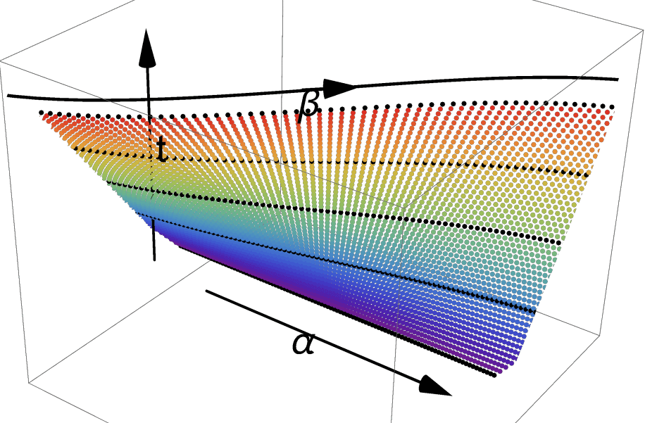
There is a nice way to visualize the idea. Imagine we slowly deform $\alpha$ into $\beta$ as time goes by. We take snapshots of the shape of the path and stack them on top of each other. The shapes of the path will trace out a surface in $2+1$ dimension. As is shown above, a straight path is deformed to a curved one. The requirement of continuousness is made clear by requiring that the surfaces that the paths trace is continuous. We can say that $F$ can be fully represented by the surface is drawn above.

Here is an animated version of the map $F$ just for fun. The code is written in Mathematica. I provide the code here if you want to play with it yourself.

Nakahara mainly used the $2$-dimension notation as below.

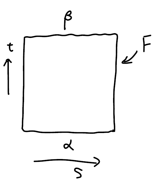
The planar diagram is to be read in this way: There are two different type of time. The first time denoted by $s$ is the time we spend traveling along some path. This $s$ parameter determines how long we spend on the path. There is also a time denoted by $t$, which signifies the which point we are during the deformation. Keep it in mind that both axis are time of different types will avoid confusion about what is deformed later in this note.

A better way to draw it would be to color map the path with the distance traveled along it, and then plot the $3$d diagram. That way we seethe entire picture on one diagram. It’s a nice thing to have, but I am running a bit short on time, so we will do without it. If you are interested you can plot it yourself or email me so we can work together.

This could be misleading in the following way, but I will include them as they provide some insight into which types of functions we should use to construct the continuous map $F$ in later times.

1. When there is actually a “deformation” happening to the actual paths as in the case $\alpha\rightarrow \beta$, the $F$ can look like an identity map.

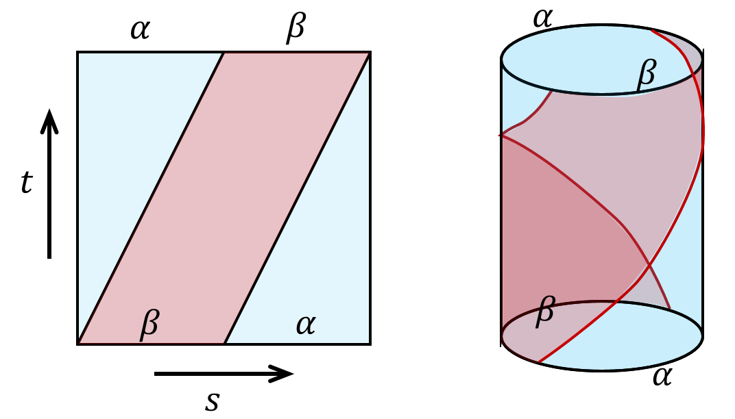
2. When there is absolutely no deformation happening to the actual path as we will see later, the $F$ can look like there is a deformation. Consider $\alpha*\beta$ and $\beta * \alpha$. The result of the same shape, but there is a twist in $F$’s planar diagram. (There are no kinks in the map $F$ if we were to represent it in $3D$. But here we have a walk-around for the planar diagram: wrap it around a cylinder to represent that $\alpha$ and $\beta$ connects to a full circle. Even then, there is no deformation happening to the shape of any of the paths.)

   

Homotopy as an Equivalence Relation

There are three requirements for a relation to be an equivalent relation, namely reflectivity, symmetry, transitivity. We will proof the one by one.

• Reflectivity

  $\alpha\sim\alpha$: Take $F(s,t)=\alpha(s), \quad\forall t$.

• Symmetry

  If $\alpha\sim\beta$, There exists $ F(s,t)$ such that $F(s,0)=\alpha(s),\ F(s,1)=\beta(s),\ F(0,t)= F(1,t)$. We have that $F(s,1-t)$ is the map $\beta\rightarrow\alpha$. This can be seen as a time reversal.

• Transitivity

  If $\alpha\substack{F _ 1\ \huge\sim}\beta$ and $\beta \substack{F _ 2\ \huge\sim} \gamma$. Then the function $F(s,t)=\cases{F _ 1(s,2t),\quad t\in (0,1/2)\F _ 2(s,2t-1),\quad t\in (1/2,1)}$ maps $\alpha$ to $\gamma$, namely $\alpha\sim\gamma$. Visually that’s equivalent of gluing the surfaces of $F _ 1$ and $F _ 2$ together.

  

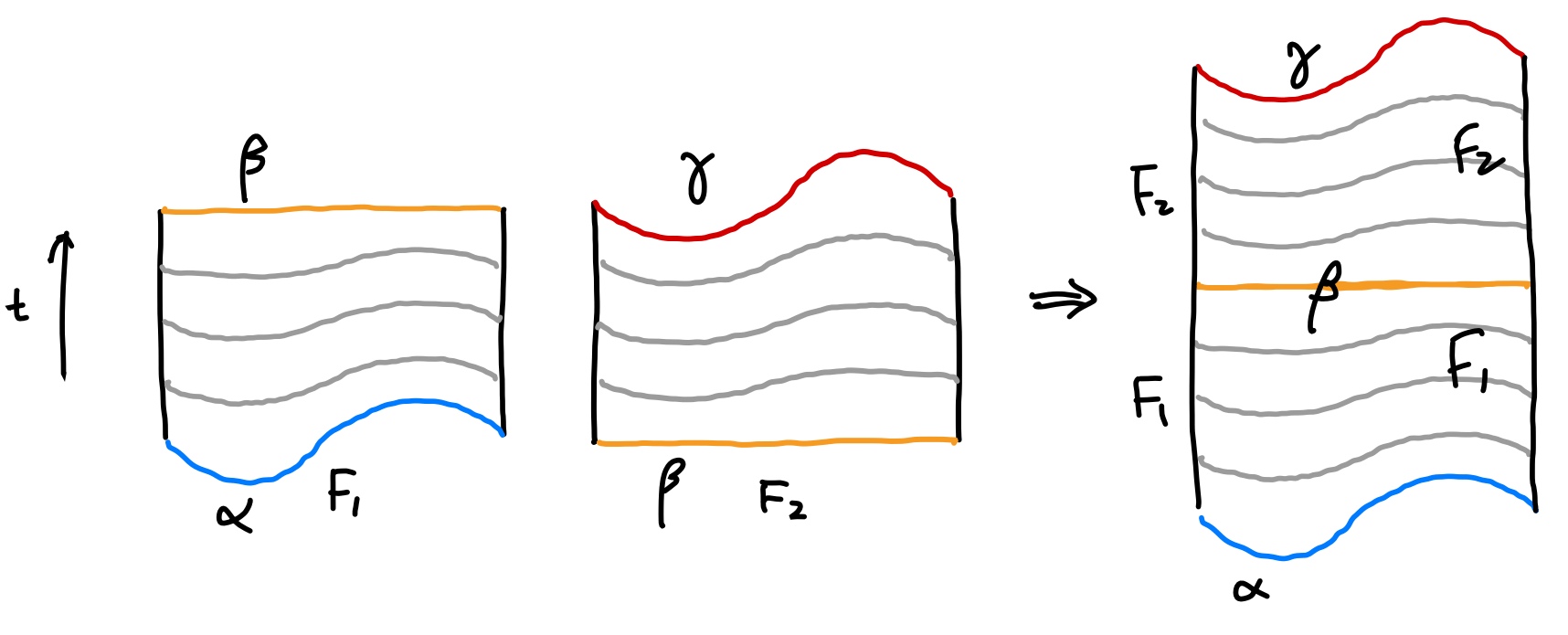
Hence by definition, homotopy is an equivalence relation.

We see that homotopy relations respects or preserves multiplication, namely, if $\alpha _ 1\substack{F _ \alpha\ \huge\sim}\alpha _ 2$, and $\beta _ 1\substack{F _ \beta\ \huge\sim}\beta _ 2$, then we have $\alpha _ 1\beta _ 1 \sim \alpha _ 2\beta _ 2$. This can be shown using the following diagram.

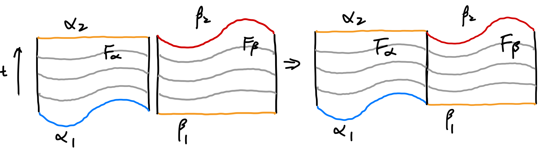
We can proof it by construction $F(s,t)=\cases{F _ 1(2s,t),\quad s\in (0,1/2)\F _ 2(2s-1,t),\quad s\in (1/2,1)}$.

Note about equivalence relation and why we need homotopy:

I imagine this is a new concept for most of the viewers of this post. So I will give some background to the notion here.

Any relation that has reflectivity, symmetry, transitivity is by definition an equivalence relation. Equality and inequalities are obvious types of equivalence. Some other equivalence relations include the famous congruence and similarity between shapes such as triangles. The equivalence relation itself is not very useful.

The equivalence relation of a set tells us that there are elements that can be seen as equivalent which enable us to define equivalent classes. This enables us to group elements that behave the same (equivalently). And we don’t have to look at every element, but the representatives of each class.

Consider the following equivalence relation defined over $\mathbb Z-{0}$:

If $a,b\in \mathbb Z$, $a+b\gt 0$, we call $a\sim b$. (This equivalence relation is such “grouping by the same sign”)

It’s evident

1. $a\sim a$.
2. If $a\sim b$, then $b\sim a$.
3. If $a\sim b$ and $b\sim c$, then $a\sim c$.

Then we have the equivalence relation $\sim$ that distinguishes two subsets of $\mathbb Z- {0}$. We denote them to be $[1]$ and $[-1]$. This information reveals the structure of the set. (It actually gives a new set with only two elements: ${[-1],[1]}$. This is sometimes denoted as $\mathbb Z- {0}/\sim$.) But still, it’s not of much use.

When we discover that the equivalence class preserves (or respects) multiplication, that’s when things become interesting. Namely we know if $a _ 1\sim a _ 2, b _ 1 \sim b _ 2$ ($a$’s are of the same sign, and so are $b$), then $a _ 1 \times a _ 2\sim b _ 1\times b _ 2$. We have new group ${[-1],[1]}$ with multiplication.

By doing so, have a new group defined from the old one. Of course, this is an equivalence relation was constructed out of a group. But in the case of homotopy, we were able to construct a group out of a set that does not have a group structure. That’s why we need to define homotopy.

Homotopy Makes Paths a Group

We will show that if we consider the set of homotopy classes instead of actual paths at base point $x _ 0$, we have a group. This group denoted as $\pi _ 1(\mathcal M, x _ 0)$, called the fundamental group.

Since the homotopy relation respects the multiplication, namely if $\alpha _ 1\substack{F _ \alpha\ \huge\sim}\alpha _ 2$, and $\beta _ 1\substack{F _ \beta\ \huge\sim}\beta _ 2$, then we have $\alpha _ 1\beta _ 1 \sim \alpha _ 2\beta _ 2$, we can define the multiplication between classes as

\[[\alpha]*[\beta]=[\alpha*\beta].\]

In other words, we can use elements from each class as representatives and whatever relation these elements have, we can always find the corresponding relations of the classes they belong by putting them to the class.

To show that the set of paths under homotopy relation does form a group, there are four requirements we need to show, namely closedness, associativity, unique unit and inverse. We will prove them one by one.

Closedness:

This is evident. A path multiplied to a path is still a path. Hence belongs to a class.

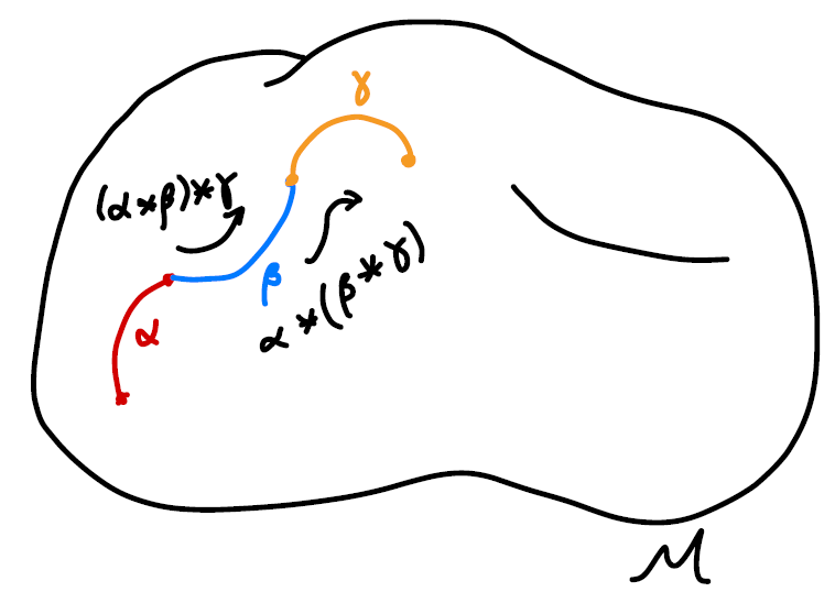
Associativity:

To prove the associativity between classes,

\[([\alpha]*[\beta])*[\gamma]=[\alpha]*([\beta]*[\gamma])\]

we can prove using the elements first.

\[\begin{align} (\alpha*\beta)(s) = \cases{ \alpha(2s), \quad s\in[0,\tfrac{1}{2}]\\ \beta(2s-1), \quad s \in[\tfrac{1}{2},1] },\quad \big((\alpha*\beta)*\gamma \big)(s) = \cases{ \alpha(4s), \quad s\in[0,\tfrac{1}{4}]\\ \beta(4s-1), \quad s\in[\tfrac{1}{4},\tfrac{1}{2}]\\ \gamma(2s-1), \quad s\in[\tfrac{1}{2},1]\\ } \\ (\beta*\gamma)(s) = \cases{ \beta(2s), \quad s\in[0,\tfrac{1}{2}]\\ \gamma(2s-1), \quad s \in[\tfrac{1}{2},1] }, \quad \big(\alpha*(\beta*\gamma) \big)(s) = \cases{ \alpha(2s), \quad s\in[0,\tfrac{1}{2}]\\ \beta(4s-2), \quad s\in[\tfrac{1}{2},\tfrac{3}{4})]\\ \gamma(4s-3), \quad s\in[\tfrac{3}{4},1]\\ } \end{align}\]

This was already evident even without the expression by looking at the results as stated before. Here we are going for a mathematical proof.

Our mission is to find a continuous map $F$ that maps from $\big((\alpha\beta)\gamma \big)$ to $\big(\alpha(\beta\gamma) \big)$. One easy way to do this is to find the following $F$ with the mapping characterized by (monotonically increasing w.r.t. $s$ for simplicity) $f _ 1$, $f _ 2$ and $f _ 3$. Note the range of the parameters of the paths are determined by the maximal of $f$s which conveniently locate at $s=1$.

\[\begin{align*} F(s,t) =\cases{ \alpha(f _ 1(s,t)), \quad s\in[0,g _ 1(t)]\\ \beta(f _ 2(s,t)), \quad s\in[g _ 1(t),g _ 2(t)]\\ \gamma(f _ 3(s,t)), \quad s\in[g _ 2(t),1]\\ } \end{align*}\]

The constraints on $g$’s are

\[\begin{array}{llll} g _ 1(0) = \tfrac{1}{4}, & g _ 1(1) =\tfrac{1}{2}\\ g _ 2(0) =\tfrac{1}{2}, & g _ 2(1) = \tfrac{3}{4}\\ \end{array}\]

The constraints on the $f$’s are defined by the the “partitions” of $\alpha$, $\beta$ and $\gamma$ at $t=0$ and $t=1$. Namely

\[\begin{array}{llll} f _ 1(s,0) = 4s, & f _ 1(s,1) = 2s, & f _ 1(0,t)=0, & f _ 1(g _ 1(t),t)=1.\\ f _ 2(s,0) = 4s-1, & f _ 2(s,1) = 4s-2.& f _ 2(g _ 1(t),t)=0, & f _ 3(g _ 2(t),t)=1\\ f _ 3(s,0) = 2s-1, & f _ 3(s,1) = 4s-3.& f _ 3(g _ 2(t),t)=0, & f _ 3(1,t)=1\\ \end{array}\]

There are obviously many choices of $f$’s and $g$’s that gives the above result, you can fit an exponential function if you want. This freedom of choice corresponds to the freedom of choices of continuously deforming the paths. For simplicity, we choose linear functions for $g$ and then find expressions for $t$.

After finding $g$, I don’t have a good way of determining the expression for $f$, other than trial and error. One hint is to look at the planar diagram of $F$. If there is a stretch, the expression is typically of the form $s/t$, else it would the linear combination of $s$ and $t$.

The result we have is

\[\begin{align*} F(s,t) =\cases{ \alpha(\frac{4s}{1+t}), \quad s\in[0,\tfrac{t+1}{4}]\\ \beta(4s-1-t), \quad s\in[\tfrac{t+1}{4},\tfrac{t+2}{4}]\\ \gamma(\frac{4s-t-2}{2-t}), \quad s\in[\tfrac{t+2}{4},1]\\ } \end{align*}\]

This map $F$ is continuous. Here are the planar diagram and $3$-dimensional representation of $F$.

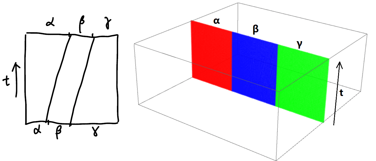
Be very careful with what this sketch represents. Again, there is absolutely no deformation if we take $\alpha$, $\beta$ and $\gamma$ as path and multiply them. You can see it by just looking at the result without the mathematical proof. The “tilted deformation” is actually the re-distribution of time spend of each path.

I actually spent 2 hours trying to visualize this deformation while writing this note. I could not wrap it around my head why every time I get a constant map instead of a nice deformation as is shown above. Then I realized that that’s exactly what we are trying to proof: geometrically the map $([\alpha][\beta])[\gamma]=[\alpha]([\beta][\gamma])$ is identity map.

Unique unit:

The unique unit element is just $c _ x: I \rightarrow x\in \mathcal M$. We need to show that

\[[\alpha] ∗ [c _ x] = [\alpha] \text{ and } [c _ x] ∗ [\alpha] = [\alpha]\]

This is shown by using

\[\begin{align*} F(s,t) =\cases{ \alpha(\frac{2s}{t}), \quad s\in[0,\tfrac{t+1}{2}]\\ x, \quad s\in[\tfrac{t+1}{2},1] } \end{align*}\]

And the planar diagram is as following

The planar diagram shows the change of time distributed on the paths, and the $3$d diagram shows what happens to the actual shape: nothing, hence the name unity.

Inverse

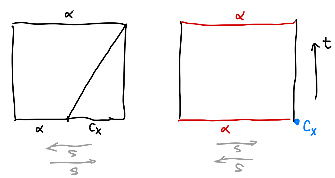
We will show that $\alpha^{-1}\alpha=\alpha\alpha^{-1}=c_x$. The homotopy map is \(F(s, t) = \cases{ \alpha(2s(1 − t)), \quad s\in[0,\tfrac{1}{2}]\\ \alpha(2(1−s)(1-t)), \quad s\in[\tfrac{1}{2},1] }\) This map gives us $\alpha^{-1}*\alpha\sim c_x$. Substitute $s$ with $1-s$ and we have the other relation. This gives us the inverse.

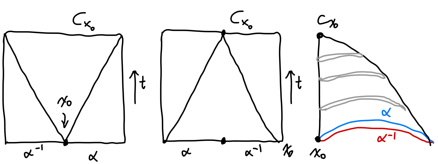
Notice that the planar diagram of $F$ can is again drawn as a square even if one of the path is a single point, since the $x$-axis correspond to traveling time along the path, rather than actual shape of it. In the left planar diagram we see that initially we spent an infinitely small amount of time at $x_0$ and spend most of the time at the two path. During the deformation, we spend less and less time on the path but spend more and more time at the starting point. Finally we spend all the time on the single point and

Notice that different orders give different planar diagrams of $F$ but the $3$d diagram does not change.

Invariance of Fundamental Group

So now we have proven that the homotopy classes of path of a manifold at a given point does constitute a group. This group is called the fundamental group of manifold $\mathcal M$ at point $x$, denoted as $\pi_1(\mathcal M , x)$. This group is also called the first homotopy group.

We have yet to prove that this fundamental group is invariant under continuous deformation. And more importantly, the fundamental group we have now is not of much use since there are infinite many choices of $x$ on a given manifold $\mathcal M$ and we don’t know which point should we use. These two problems will be addressed in this section.

Both of the proof is related to the equivalent classes defined before.

Invariance under Continuous Deformation

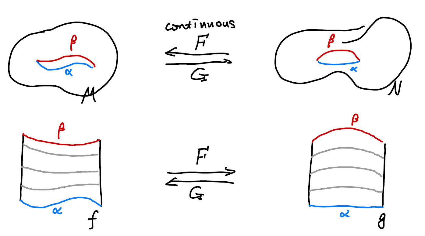
Let’s say there is a way to continuously deform a manifold $\mathcal M$ to $\mathcal N$, the map denoted as $\mathbb F$, and a map from $\mathcal N$ back to $\mathcal M$, denoted $\mathbb G$. The map $\mathbb F$ is called the homotopy equivalence and $\mathbb G$ its inverse. We call $\mathcal M$ and $\mathcal N$ “of the same homotopy type”, which we will assert without proof to be a equivalence relation.

Theorem: Let $\mathcal M$ and $\mathcal N$ be topological spaces of the same homotopy type. If $f \ : \mathcal M \rightarrow \mathcal N$ is a homotopy equivalence, $\pi_1(\mathcal M, x_0)$ is isomorphic to $\pi_1(\mathcal N, f(x_0))$.

Nakahara did not gave a proof in his book, but we can use the following diagram to understand it. If we deform the manifold continuously, we can also deform the maps between paths as well. The deformation of a map is reflected by the deformation of the surface that represent it.

Note that here I did not show the difference between the homeomorphism and homotopy. Nor have I showed why do we need a reverse homotopy map to establish a homotopy equivalence.

Invariance of Choice of Base Point

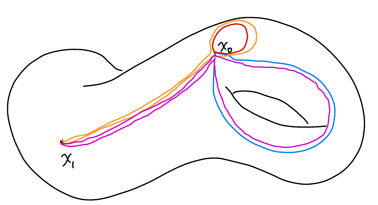
For a arcwise connected manifold (in oversimplification, we are considering one chunk of manifold instead of say two separated doughnuts), it’s easy to prove that fundamental groups at different base points are isomorphic. The map we use to construct the isomorphism is
\(P(\alpha) = \eta * \alpha *\eta^{-1}\) where $\eta(0) = x_1, \eta(1) = x_0$.

The map basically stretches the loops at $x_0$ to $x_1$. We can show that this map is one to one and is onto.

Calculation of Fundamental Groups

(From a heuristic point of view, this chapter can be moved to the beginning for a clearer picture.)

So far, we have successfully found an topological invariant that’s a group. The problem we have right now is that how can we rigorously enumerate all the homotopy classes to form this group? How can we calculate the group for a given manifold? What are some of the examples?

Edge Paths

I am going to skip the part where we calculate the fundamental groups of manifolds directly. You can find that on Nakahara. We will calculate the fundamental groups using polyhedrons. First, like in the case of smooth manifolds, we are going to define the paths on edges.

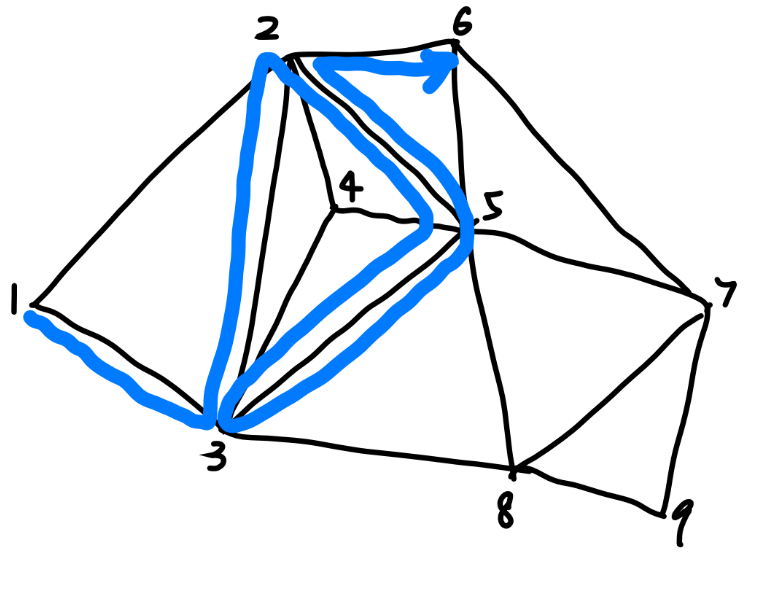
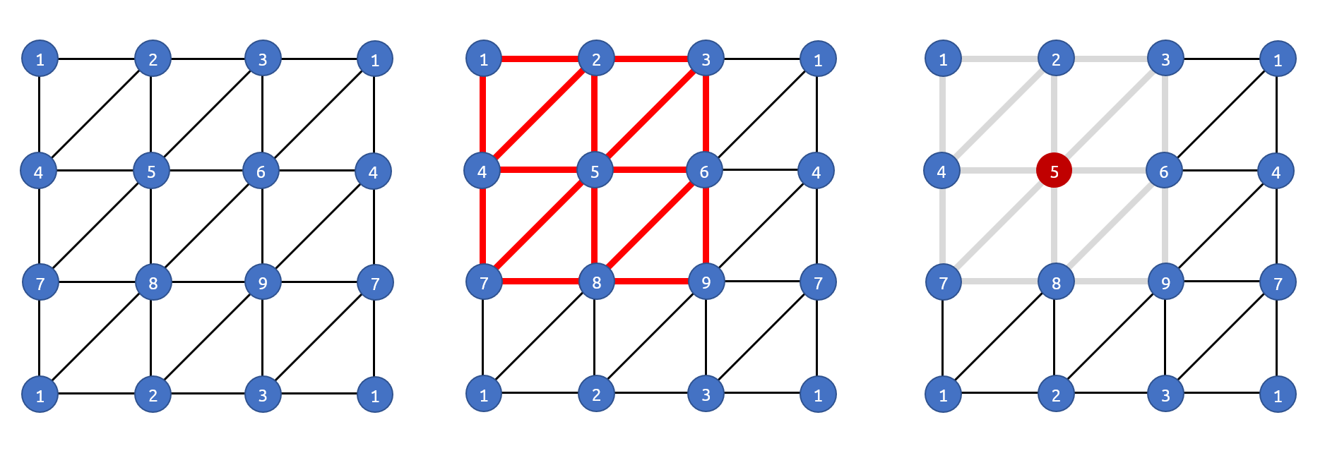
We will label the vertices (or nodes) and represent the edges (or links) as $g_{12}$. A path can be represented by a string of edges or a string of vertices. The following notations \(g_{13}g_{32}g_{25}g_{53}g_{35}g_{52}g_{26} \\ 13322553355226\) both represent the path colored in blue. We allow back travelling and looping in our definition.

Contractions of Edge Paths

Obviously there are infinite number s of path, but our first job is to limit the path to the “simplest” ones. To do that, we define two local ways to “smoothen” the path.

Polygon Paths as a Group

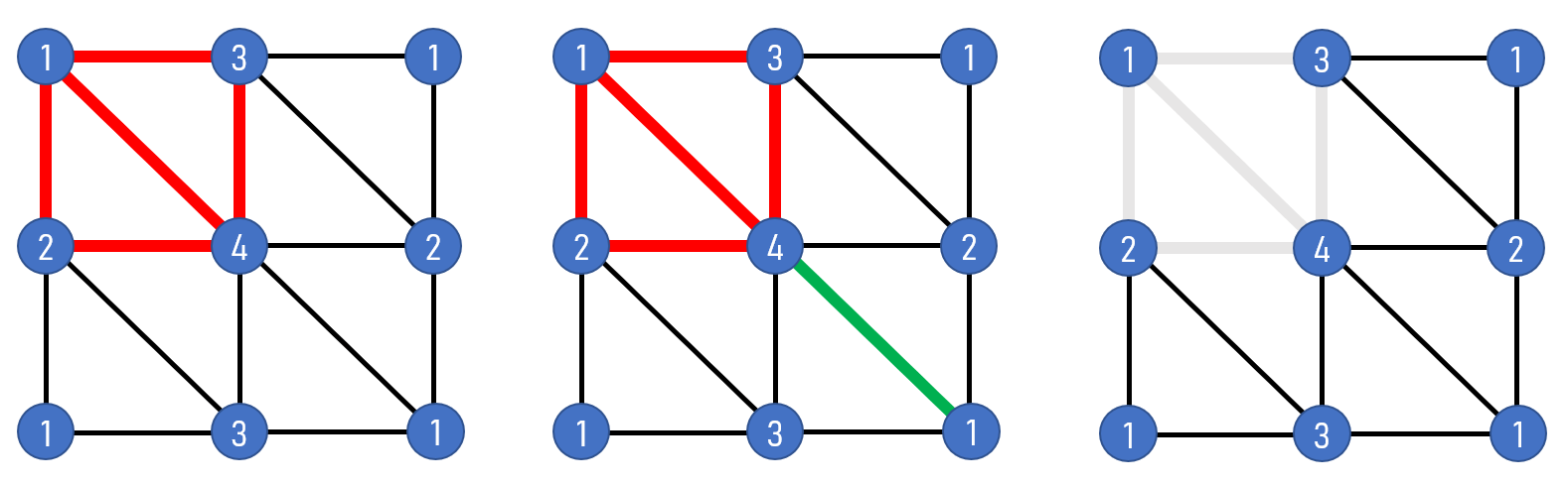
Maximal Tree of a Polyhedron

Torus’ Triangulation as Example

Non-Regular Triangulation’s Fundamental Groups