---

\[\newcommand{\bra}[1]{\left\langle{#1}\right\vert } \newcommand{\ket}[1]{\left\vert {#1}\right\rangle} \newcommand{\braket}[2]{\left\langle {#1} \, \middle\vert \,{#2} \right\rangle } \newcommand{\d}{\mathrm{d}} \newcommand{\R}{\mathbb{R}} \newcommand{\C}{\mathbb{C}} \newcommand{\K}{\mathbb{K}} \newcommand{\D}[2]{\frac{\d {#1}}{\d {#2} }} \newcommand{\Partial}[2]{\frac{\partial {#1} }{\partial {#2} }} \newcommand{\op}{\hat} \newcommand{\uvec}{\hat} \newcommand{\dfdas}{:=} \newcommand{\Eqn}[1]{\text{(Eqn. }\ref{#1}\text{)}} \newcommand{\vard}{\mathfrak{d}} \newcommand{\vare}{\mathfrak{e}} \newcommand{\e}{\mathrm{e}} \newcommand{\i}{\mathrm{i}} \newcommand{\norm}[1]{\left\vert{#1}\right\vert} \newcommand{\set}[1]{\left\lbrace {#1}\right\rbrace} \newcommand{\comm}[2]{\left[ #1 , \, #2 \right]} \newcommand{\slot}{\,\cdot\,} \newcommand{\lact}{\triangleright} \newcommand{\ract}{\triangleleft} \newcommand{\vac}{1\!\!\!\mathsf{\phantom{I}I}} \newcommand{\la}{\mathfrak} \newcommand{\anti}{\overline} \notag\]

Properties of Anyons

Fermions and Bosons

Fermions and Bosons are familiar concepts in statistics. Statistics means that more than one particle is present in the system. When exchanged, Bosonic system’s wavefunction remains unchanged while the Fermionic system’s wavefunction gains an additional minus sign. The above results are the solutions of the equation $\lambda^2=1$. Because obviously, exchange two particles twice are equivalent to no exchange.

Anyons’ Statistical Property

When we consider particles in $2+1$ dimension space, we find that things are quite different.

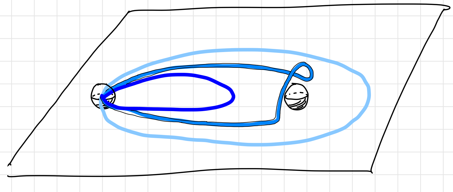
Twice exchange of two particles is equivalent to circling one particle around another. When space is $3$-dimensional, the path can shrink to a single point as is shown below. That gives the equation $\lambda^2=1$, which is the case of Fermions and Bosons. While on $2$-dimensional space, the light-blue path cannot shrink to the dark-blue path since they are topologically inequivalent. That means $\lambda^2\neq1$. Such encircling can result in a complex phase factor¹ rather than simply $\pm 1$.

A Note on the Lattice

To make the braiding topological rather than a simple permutation, the lattice needs to have a non-trivial topological characteristic. In my understanding, such connection is made by Witten’s work which connected Chern Simons theory with the knot and link invariants of Jones and Kauffman (from[^3] in Section II.A.1).

General Settings of Anyons Braiding

From now on, the existence of anyons is assumed, the experimental detail of anyons ignored. This post will focus on how these anyons can be manipulated and give desired results as a useful topological quantum computer. Anyons in our model permit the following manipulations.

1. Anyons can be created or annihilated in a pairwise fashion. (Initialization and measurement)
2. Anyons can be fused to form other types of anyons. (manipulation and measurement)
3. Anyons can be exchanged adiabatically. (manipulation)

In short, anyons are just like a “real world particle” such as electrons and positrons that can undergo creation, annihilation, and are free to move around each other.

Anyons do not decay, but the reverse process of fusion, called “fission” can be thought as the decay of anyons.

Properties of Anyons

To define an anyon model, the types of anyons must be listed. Anyons are characterized by there topological charges, sometimes this charge is simply called the label. There will always be a trivial particle called the vacuum, labeled as $\vac$. Notice that $\vac$ does not necessarily correspond to actual vacuum (as in “vacuum without anyons”). $\vac$ can represent a trivial particle such as a boson which is topologically trivial.

The anyon model is denoted by a set of particles as

\[M=\set{\vac,a,b,c,\cdots},\quad \text{$a,b,c,\cdots\,$ are distinct particles}.\]

Sometimes the antiparticle of particle $a$ will be denoted as $\anti a$.

Fusion Channels

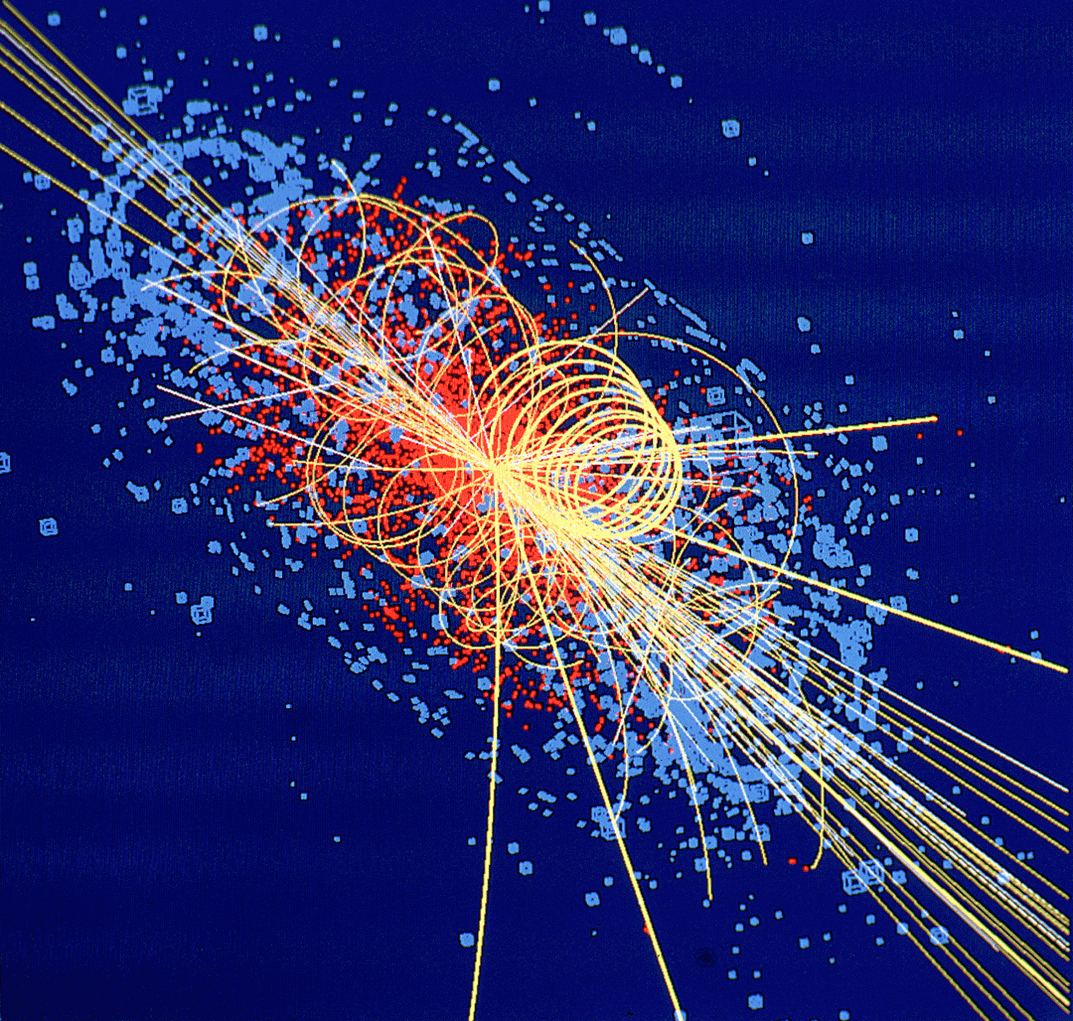
Two anyons can fuse together, just like particles in a collider can violently collide and shatter into other particles, and possible results can arise. For example, two protons might collide to two $K^+$ particles, or two $\pi^+$ particles, denoted as $pp\rightarrow K^+K^+$, $pp\rightarrow \pi^+\pi^+$ respectively, along with many other possibilities. In high energy physics, a particular result is called a decay channel. To find out about a fusion channel, you can go to PDG (thanks Yifei for teaching me that).

Two anyons can also gently fuse together to give birth to a new particle(s). Like in the case of LHC, there could be several possible outcomes for two fused particles. denoted as

\[a\times b = \sum N_{ab}^c c.\]

such that

\[a\times b = b \times a \quad \text{and}\quad a \times \vac = a\]

Adopting the term “decay channel” in high energy physics, a particular result of the fusion is called a “fusion channel”.

Fusion is also independent of order, i.e.,

\[(a\times b )\times c = a \times (b \times c)\]

Interpretation of Fusion Equations

For example, $\sigma\times \sigma = \vac + \psi$ means that two $\sigma$ anyons can be fused together, the result is either a $\psi$ particle, or (not and) a $\vac$ vacuum.

Notice that $N_{ab}^c$ is not necessarily $1$. Like in for two particles might fuse into more particles, for example, $\alpha \times \beta = 2\theta + 3\gamma$.

$\alpha \times \beta = 2\theta + 3\gamma$ means an $\alpha$ anyon can fuse with a $\beta$ anyon, the result is either one $\theta$ anyon, or one $\gamma$ anyon. The result is NOT two $\theta$ anyons, and three $\gamma$ anyons. The number serves as a way to indicate the relative possibility of a certain outcome, for the equation can be read as $\alpha \times \beta = \theta + \theta + \gamma+ \gamma+ \gamma$ . However, such scenario is not discussed in this post.

The notation of $\otimes$ and $\oplus$ is sometimes used to make such distinction, as is in ². To make my life easier, I am going to stick to $\times$ and $+$. Just bear it in mind that $\times$ means fusion, not “times”; $+$ is a notation to list possible channels, not “plus”.

We can think of fusion as a measurement in the sense that

1. Fusion channels are mutually exclusive in the sense that you can only fuse to either one of the channels. There is no superposition in the expression $\sigma\times \sigma=\vac+\psi$.
2. Repeated fusions of the same two anyons do not necessarily result in an anyon of the same type: the resulting anyons may be of several different types each with certain probabilities (determined by the theory). (See Sec. 2.2 of ²)

Braiding Rules

Below is a schematic diagram of three anyons (quasiparticles) braided on a $2$D lattice. To maintain consistency with Pachos’ book³, evolution starts from the top.⁴

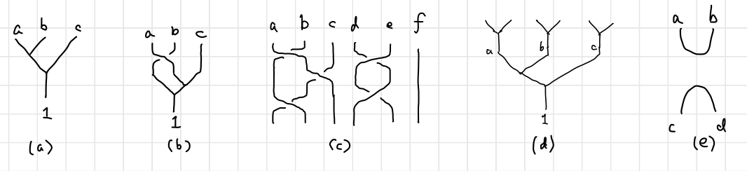
A more abstract and simpler diagram is often used as below. A $\scriptsize\boxed{\substack{\diagdown\,\,\, \diagup \newline \diagup \newline \swarrow\,\,\, \searrow } }$ diagram represents a counter-clockwise exchange, while a $\scriptsize\boxed{\substack{\diagdown\,\,\, \diagup \newline \diagdown \newline \swarrow\,\,\, \searrow } }$ represents a counter-clockwise exchange. When two lines meet together, two particles are fused together. The height indicates the order of fusion like in (a), $a$ and $b$ are fused first. Sometimes fusion are omitted to emphasize on the braiding, as is in (c). Since an antiparticle travelling forwards in time is indistinguishable from the corresponding particle travelling backwards in time, diagram as (e) is possible. However, I am not going to concern such situation in this post.

The diagram is hard to write within a document. The fusion diagram is often written in a string inside a bra or a ket, called the fusion states.

\[\ket{(ab);c},\ \ket{(ab);ba;c},\ \ket{(ab)c;(ba)c;ic;d},\ \ket{a(bc);ai;d}, \textit{ etc.}\]

The semicolon means different “stages” as time goes forward. The parentheses indicate a braiding or a fusion between the two anyons inside, and the action is inferred from the two consecutive stages. Sometimes the parentheses are dropped when there is no possible confusions, such as $\ket{ab;c}$.

Algebraic Relations Between Diagrams

Prelude of $F$-Matrices: Fusion States, Anyonic Hilbert Space

Superpositions in Fusion Diagram

To have a better understanding of $F$-matrices, we need to consider creating superposition in fusion diagrams.

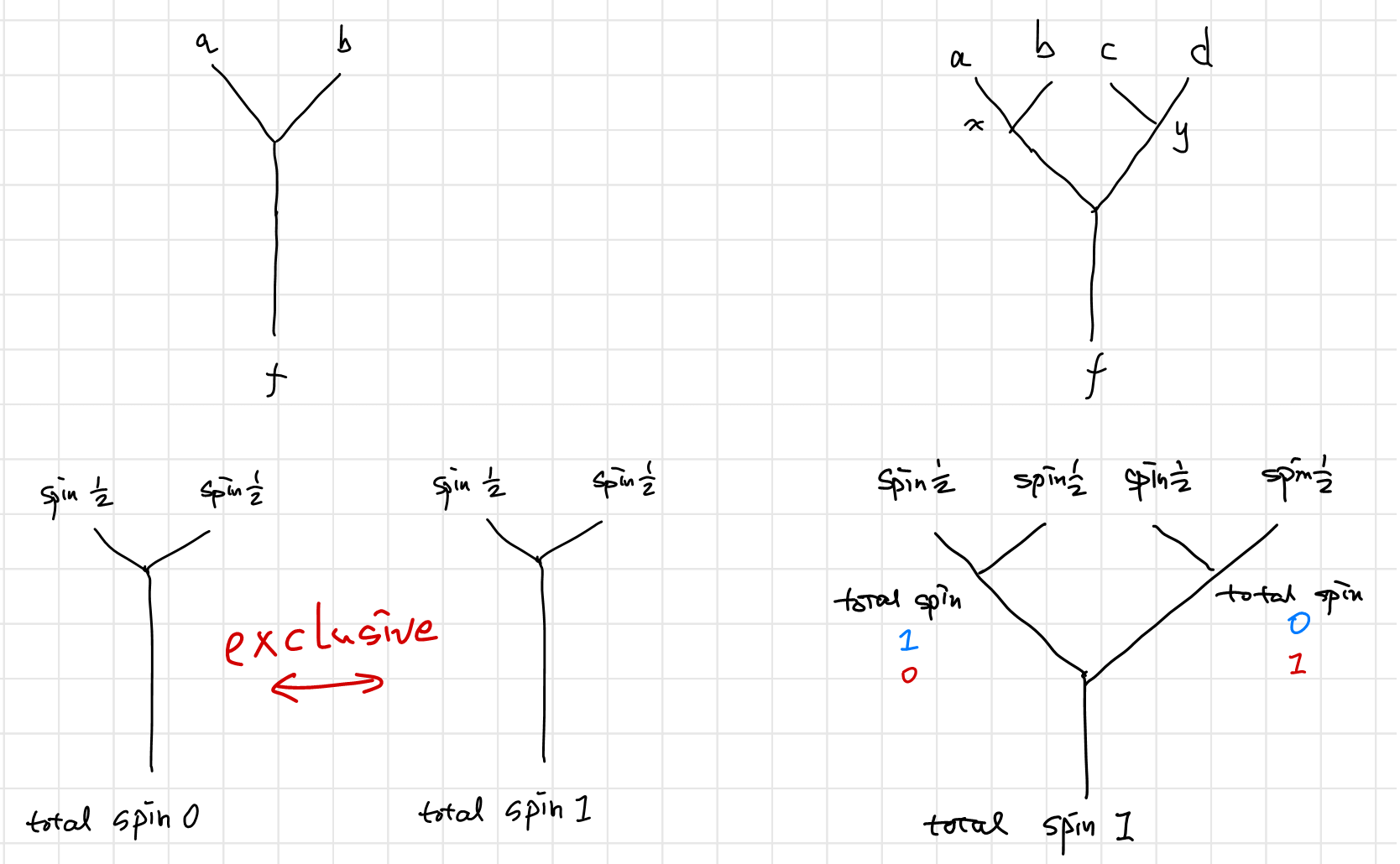
As is stated in the last chapter, fusion is much like a measurement. If two anyons are fused to a certain type of anyon, there will be no superposition between different fusion channels. Much like the total spin of two spin-half particles: once you have measured the total spin, everything is deterministic. The total spin is not in the superposition of both $0$ and $1$, it can only be either. There is no room for probabilities of different outcomes. However, when there are more than two anyons present in the fusion, the information of the intermediate result is not always determinant. Like to total spin of four spin-half particles. If the total spin is $1$, the total spin of the first pair and that of the second pair is in the superposition of two possibilities.

Spin “Fusion” Diagrams

Consider four angular momentums (spins) forming a total spin. How many ways for them to combine to a certain total spin? Two ways. $LS$ coupling and $jj$ coupling. If we consider “coupling” as fusion, we can draw the following “coupling diagram”:

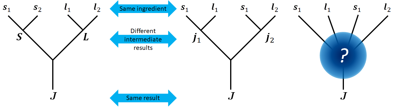
Notice that an $LS$ coupling can be written as $\ket{L,S,J}$, while $jj$ coupling will be written as $\ket{j_1,j_2,J}$. These two sets of states span the same Hilbert space, and are related to each other by Clebsch–Gordan coefficients.

If we only care about the result of a given configuration of spins and orbital angular momenta, we can draw a diagram like the one on the far right. And we can assert with confidence that either way of coupling is “correct” in describing the “fusion” result. To write in the form of fusion state, that would be $\ket{(s_1s_2)(l_1l_2);(SL);J}$ and $\ket{(s_1l_1)(s_2l_2);(j_1j_2);J}$.

Now if we consider three spins in the “fusion” order of $\ket{(s_1s_2)s_3;(S_{12}s_3);S}$ and $\ket{s_1(s_2s_3);(s_1S_{23});S}$ respectively, we will have the following diagrams.

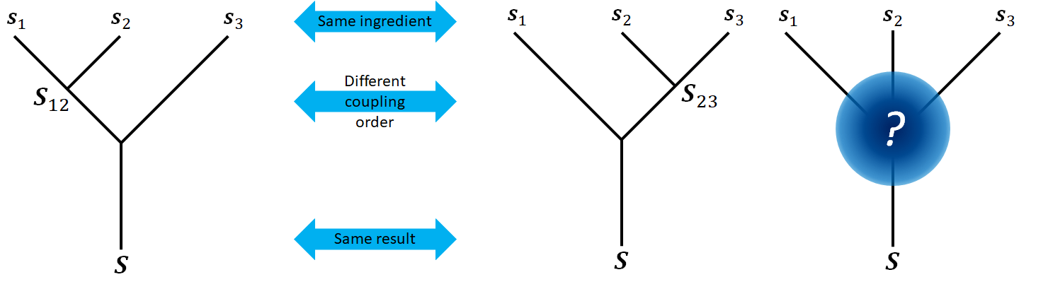
Like before, these two sets of state vectors span the same Hilbert space, where three spins are coupled as one total spin $S$. Although it’s obvious from the fact that they span the Hilbert space, I want to make this point explicitly that the state vectors of the form $\ket{s_1(s_2s_3);s_1S_{23};S}$ are orthogonal to each other. Different value of $S_{23}$ will correspond to distinguishable states, hence these states are orthogonal.

Why I wrote this subsection:

As you will see in the following sections, in $R$-matrices, the fusion states $\ket{ab;c}$ are just like actual wavefunctions of anyons: when exchanged, an additional phase factor arises. Such wavefunction of a quasiparticle is normally denoted as $\ket a \rightarrow \e ^{\imath \pi/n}\ket a$. While in $F$-matrices, such interpretation will be problematic. Of course, you can see fusion states $\ket{ab;c}$ merely a fancy way to show a wavefunction of a quasiparticle $c$, whose phase factor is determined by its origin, as $\e ^{\imath\varphi}\ket c=\ket{ab;c}$. But we further demand that the state $\ket{a(bc);ae;d}$ and state $\ket{a(bc);af;d}$ are orthogonal, and there is a unitary transformation between two sets of basis $\set{\ket{a(bc);a_;d}}$ and $\set{\ket{(ab)c;_c;d}}$.

The question remains unanswered. What are the states written as $\ket{ab;c}$, or even more fancily denoted as $\ket{\substack{a \quad b\newline \diagdown\diagup\newline \mid \newline c}}$? Are these states merely wavefunctions in quantum mechanics? As is stated in ³, the fusion states have to correspond to certain quantum states of the constituent particles.

I struggled a lot when I first studied TQC. I just couldn’t convince myself that such states are orthogonal. Then I read in ¹:

Recall that in $\mathrm{SU}(2)$, there are multiple states in which spins $j_1$, $j_2$, $j_3$ couple to form a total spin $J$. For instance, $j_1$ and $j_2$ can add to form $j_12$, which can then add with $j_3$ to give $J$. The eigenstates of $\vert j_{12}\vert^2$ form a basis of the different states with fixed $j_1$, $j_2$, $j_3$, and $J$. Alternatively, $j_2$ and $j_3$ can add to form $j_{23}$, which can then add with $j_1$ to give $J$. The eigenstates of $\vert j_{23}\vert^2$ form a different basis. The $6$$j$ symbol gives the basis change between the two.

I wrote this section so the idea of different fusion states is orthogonal to each other wouldn’t seem so abrupt to readers who are new to this field. I sure spend a lot of time struggle with it.

A Word on Fusion

When you consider anyons fusion, how exactly do they fuse in your mind? Do you picture the fusion as two particles violently smash to each other, crashing into debris, or do you picture the process as two drops of water merge into one bigger drop of water?

The fusion of anyons can be neither. Two anyons close together, away from each other can be efficiently considered as fused. In this case, the fusion is more like an anyonic party where some of the anyons pair together dancing in distinct rhythms, while others walking around talking to each other as “braiding”. Just like when two electrons are brought together and isolated, they behave exactly like a single new spin, but the two electrons are not smashing nor merging into each other. They stay perfectly as individual particles.

In this light, our fusion state $\ket{a(bc);ae;d}$ can be seen as the wavefunction of three anyons $a$, $b$ and $c$, whose collective behavior is the same as anyon $d$. Such interpretation provide us with a connection from the fusion Hilbert space to the familiar multi-body particle Hilbert space.

$F$-Matrices

After a long prelude, I hope you can still remember the title of this chapter: “Algebraic Relations Between Diagrams”. We are going to find out the algebraic relations between fusion diagrams. The first one being $F$-matrices.

The fusion is associative, i.e.

\[(a\times b)\times c = a\times (b\times c)\]

The associativity is captured by the $F$-matrix.

Just like the case of three spins, left-most-first fusion states span the same Hilbert space as the right-most-first fusion states. $F$-matrix is the representation transformation matrix between these two bases. And as bases, the left-most-first fusion states are orthogonal to each other, and or are the right-most-first fusion states.

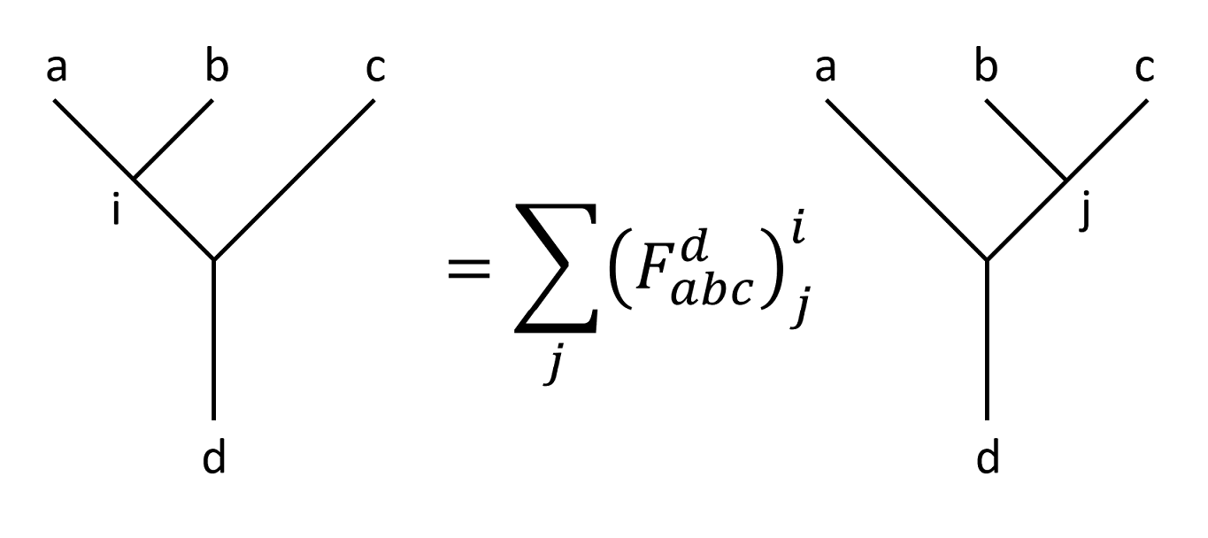
Write that in the form of fusion states, we have

\[\ket{(ab)c;ic;d}=\sum_j\left(F_{abc}^d\right)^i_j\ket{a(bc);aj;d}.\]

Of course the above equation can be revered, as

\[\ket{a(bc);aj;d}=\sum_i\left({F_{abc}^d}^{-1}\right)^j_i\ket{(ab)c;ic;d},\]

where the convention is that an $F$-matrix represents the representation transformation from right-most-first fusion to left-most-first fusion (which is called a canonical fusion), and an $F^{-1}$-matrix represents the reverse.

On some literature, you will see $F$-matrix noted as $F_d^{abc}$, which is in accordance with the orientation of the fusion tree. Why am I not using this notation, you ask. That’s because I used Pachos’ book as main reference, and it was too late for me to change my notation. Let this be a lesson.

$R$-Matrices

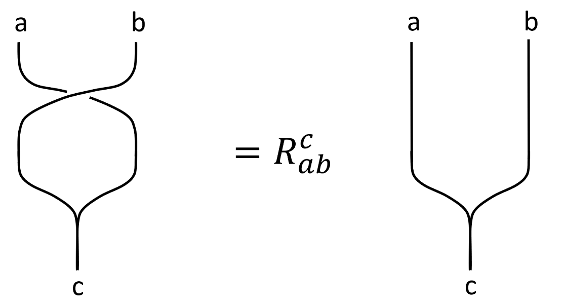
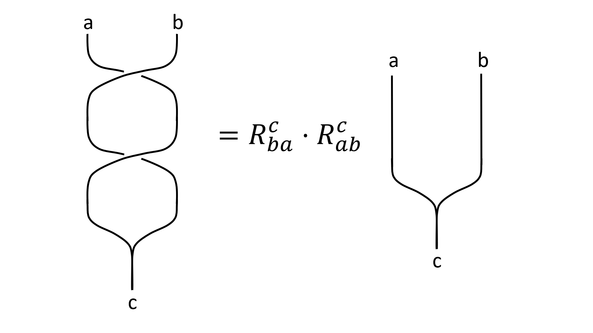
$R$-matrices are pretty easy to understand, as they describe the defining property of anyons: when exchanged, a non-trivial phase factor (matrix) is present.

Notice that $R_{ab}^c$ is not necessarily the inverse to $R_{ba}^c$, since an exchange of two anyons does not necessarily return to the original state.

Pentagon Equation

Given a fusion diagram, it is possible to transform or simplify it using $R$-moves and $F$-moves. You can imagine that we can unwind an intertwined fusion diagram in a boring-looking diagram with a lot $F$-matrices and $R$-matrices multiplied. This is nothing more than a complicated representation transformation between the fusion states $\ket{1234;\ \dots\ ;5}$.

We can even make a full circle of such transformations. In other words, there exists two path to transform a fusion tree to another. One of such transformation is characterized by the pentagon equation (or pentagon identity).

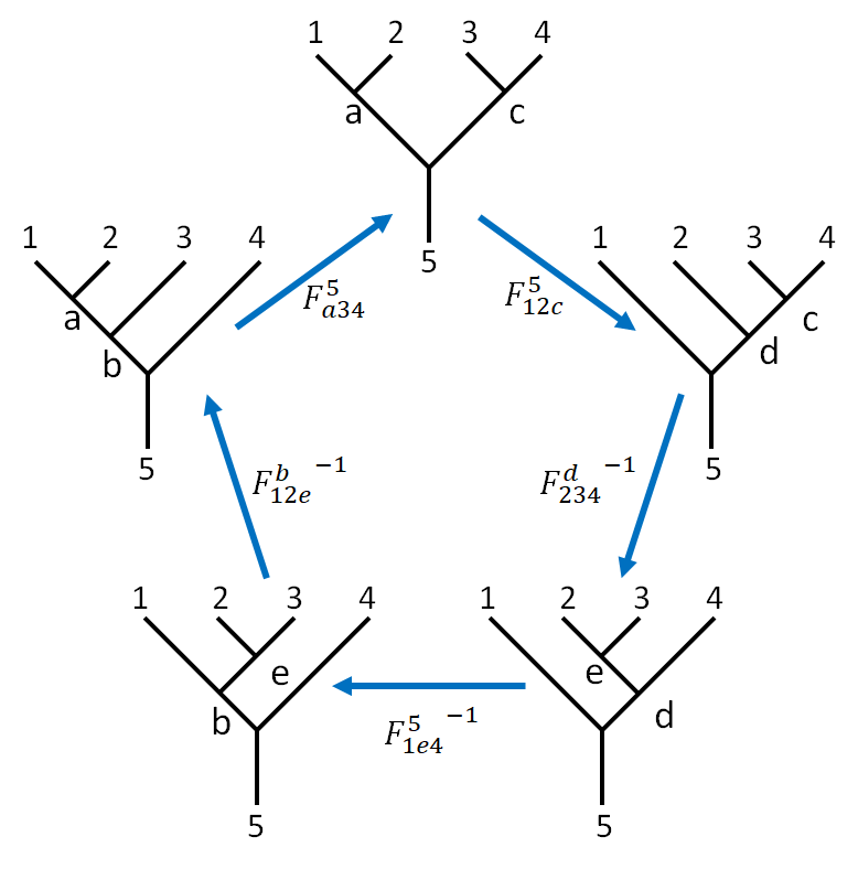
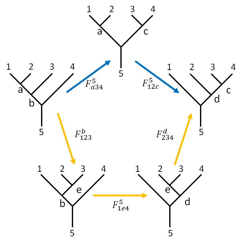
This picture adopted from ³ is quite self-explanatory. With some effort, we can write the element-wise equations clockwise starting from the canonical fusion.

\[\begin{array}{} &&&\ket{a34;b4} &= \sum_c \left(F_{a34}^5\right)_c^b \ket{a34;ac} \\ &&&\ket{a34;ac} &= \sum_d \left(F_{12c}^5\right)_d^a \ket{12c;dc} \\ \ket{12c;dc} &= \sum_e \left({F_{234}^d}^{-1}\right)_e^c \ket{1e4;1d} & \rightarrow & \ket{1e4;1d} &= \sum_c \left(F_{234}^d\right)_c^e \ket{12c;dc} \\ \ket{1e4;1d} &= \sum_b \left({F_{a34}^5}^{-1}\right)_b^c \ket{1e4;b4} & \rightarrow & \ket{1e4;b4} &= \sum_d \left(F_{1e4}^5\right)_d^b \ket{1e4;1d} \\ \ket{1e4;b4} &= \sum_e \left({F_{123}^b}^{-1}\right)_d^b \ket{a34;b4} & \rightarrow & \ket{a34;b4} &= \sum_e \left(F_{123}^b\right)_e^a \ket{1e4;b4} \end{array}\]

Where leading term “$1234;$” and the ending term “$;5$” part of fusion state $\ket{1234;a34;b4;5}$ are omitted, so that would become $\ket{a34;b4}$.

Combine the above equations, we have

\[\ket{a34;b4} =\sum_c \sum_d \left(F_{a34}^5\right)_c^b \left(F_{12c}^5\right)_d^a \ket{12c;dc} \\\ket{a34;b4}= \sum_e \sum_d \sum_c \left(F_{123}^b\right)_e^a \left(F_{1e4}^5\right)_d^b \left(F_{234}^d\right)_c^e \ket{12c;dc}\]

Thus the pentagon identity is

\[\left(F_{a34}^5\right)_c^b \left(F_{12c}^5\right)_d^a = \sum_e \left(F_{123}^b\right)_e^a \left(F_{1e4}^5\right)_d^b \left(F_{234}^d\right)_c^e\]

The abandonment of super- and subscripts look daunting, but the equation will be drastically simplified if there are only a few ($2$ for Fibonacci , $3$ for Ising) anyons in the model, which we will see later.

Hexagon Equation

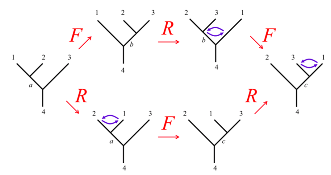
There is another kind of transformation which involves both $F$ and $R$ matrices. The identity is called the hexagon identity, as is pictured as below. To be concise, the transformation does not go around a circle to avoid unwanted inverses of matrices. The “active” part during each part is circled out. The initial arrangement of anyons are always $123$, and intermediate arrangements are labeled in red.

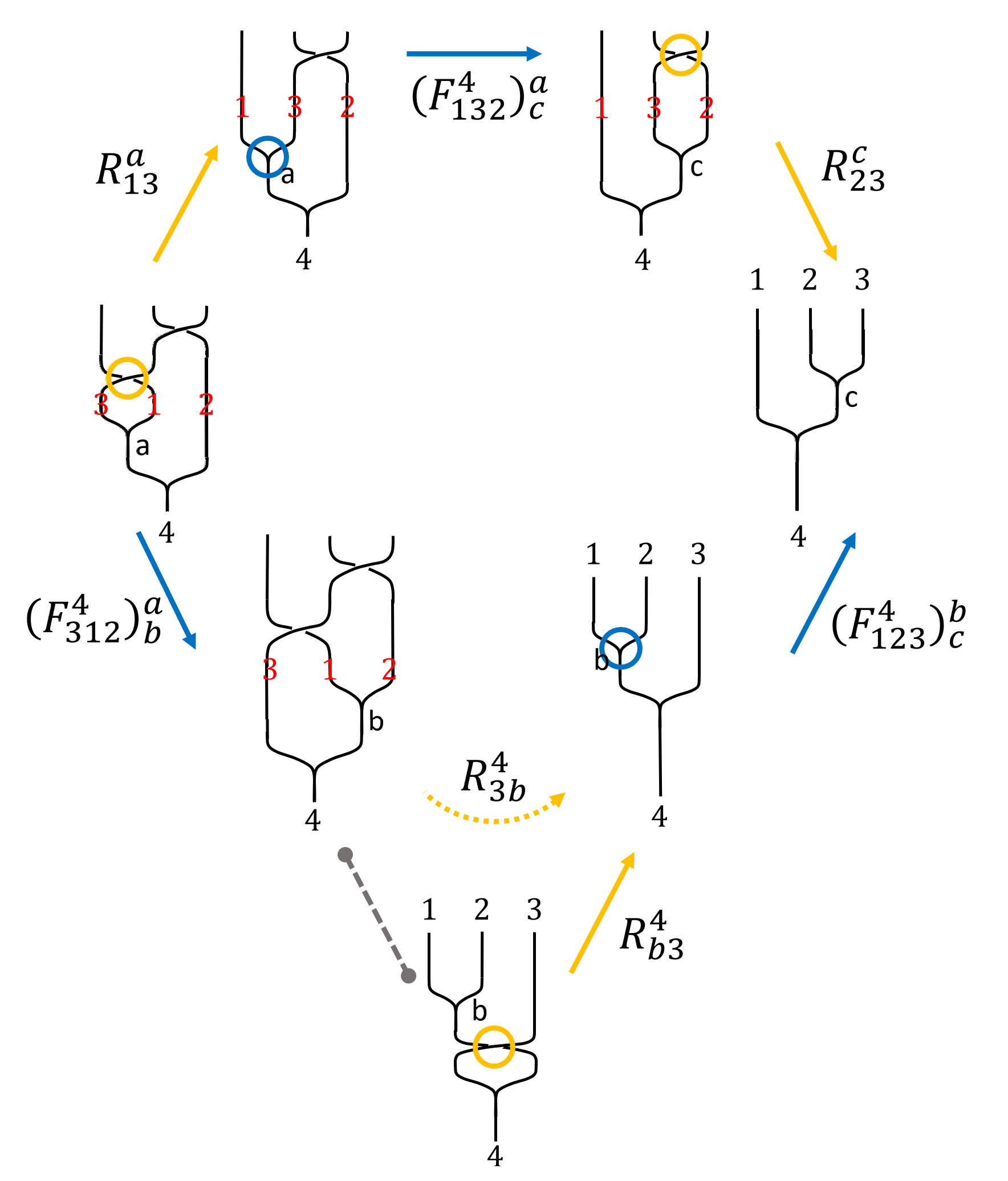
This picture adopted from² is quite self-explanatory. Notice that the gif in the lower right corner shows that just like strands in our daily life, we can gently move them is they are not intertwined. Notice that the order of the fused anyons are not changed. This version of hexagon diagram I will call as Simon’s version.

Note on morph:

1. Morph an important step in hexagon identities. I was baffled when I was writing this post.

   

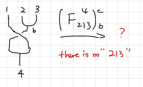
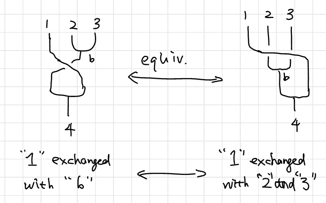
2. If the order of the initial anyons are changed, there should be extra $R$-matrices, even if there is a way to obtain the same result. One of such incorrect ways to morph is shown below. (As you might have guessed, I discovered it after I made the mistake.)

1. The morph actually says a lot about what the fusion is. From the diagram below you see that a fused anyon $b$ is actually equivalent to the direct package of $2$ and $3$ as individuals.

   

There is also other versions of hexagon identity, as is shown below (picture taken from this slide show) where Pachos’ book is using. As you can probably see, this version’s fusion tree are flipped horizontally, as by ⁵: “Particularly, there is another family of hexagons obtained by replacing all righthanded braids with left-handed ones. In general, these two families of hexagons are independent of each other.”

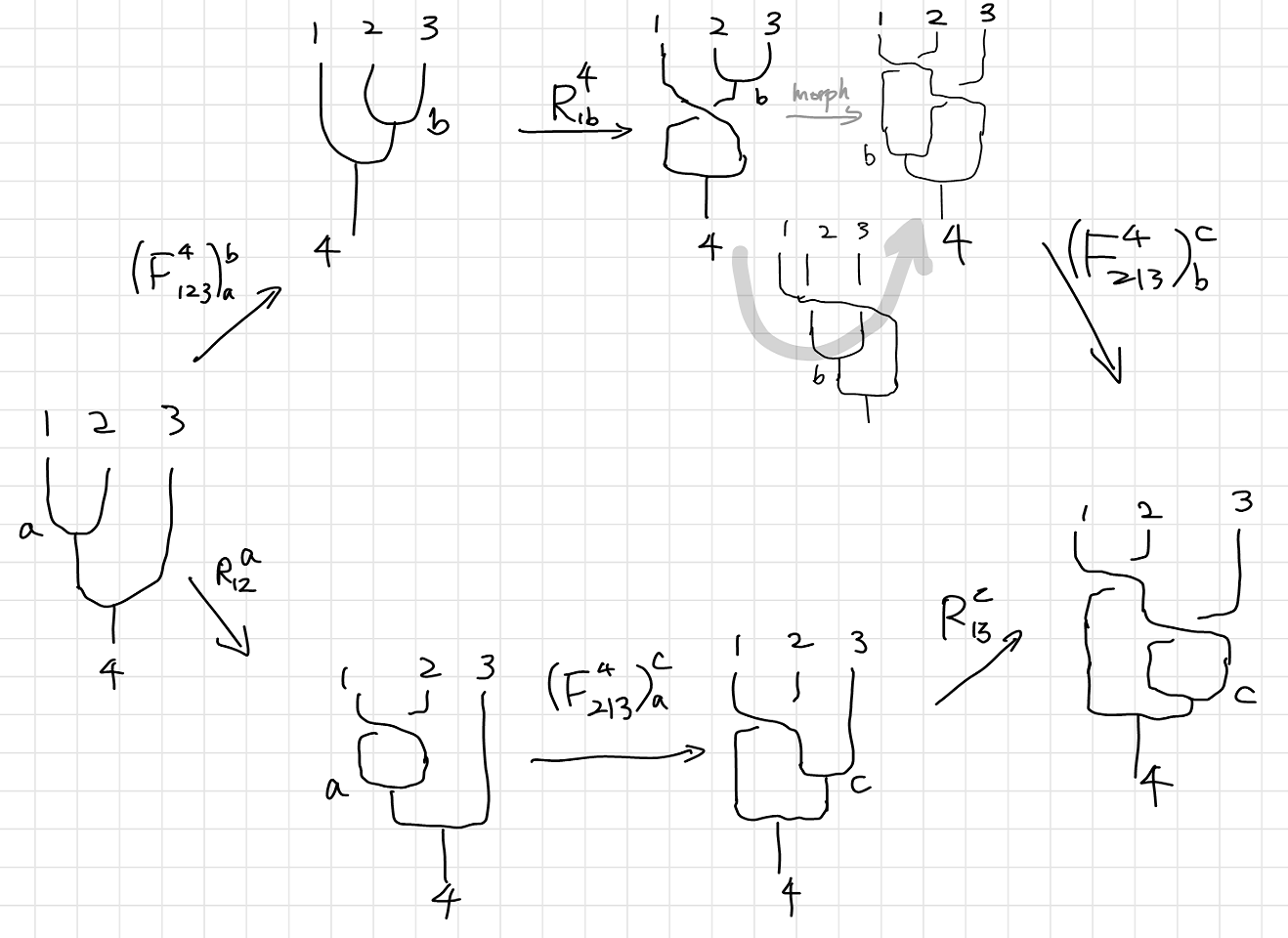
Hence using the same technique before if you are not quite familiar with it. Personally I prefer to note the coefficients on the diagram so I don’t have to go through the hassle. We can write down (a version of) hexagon identity as

\[\begin{array}{} \sum_b \left(F_{312}^4\right)_b^a R_{3b}^4 \left(F_{123}^4 \right)_c^b = R_{13}^a \left(F_{132}^4\right)_c^a R_{23}^c & \text{Simon's version.}\\ \sum_b \left(F_{231}^4\right)_b^c R_{1b}^4 \left(F_{123}^4 \right)_a^b = R_{13}^c \left(F_{213}^{4}\right)_a^c R_{12}^a &\text{Pachos' version}. \end{array}\]

Again, the abandonment of super- and subscripts look daunting, but the equation will be drastically simplified if there are only a few ($2$ for Fibonacci , $3$ for Ising) anyons in the model, which we will see later.

Notes on the Complexity of Pentagon and Hexagon Equations

The pentagon and hexagon equations looks very complicated. Once we apply the equations to actual models, things will become drastically simplified. Fibonacci anyons and Ising anyons contains a very limited types of anyons, and many of the $F$-matrices are trivial. We will see that in the upcoming notes of case study.

Notes on the Pentagon and Hexagon Equations

As is stated in ¹, we can solve for the $F$-matrix and $R$-matrix directly from the pentagon and hexagon equations. The only information a specific anyon model can provide is in the fusion equation $a\times b = \sum N_{ab}^c c$. For example, the $F$-matrices for Fibonacci anyons are solved from pentagon equation in⁵.

Also, $F$- and $R$-matrices can be viewed from modular tensor category, which I am not familiar with at all now.

Why is it necessary to invoke category theory simply to specify the topological properties of non-Abelian anyons?Could the braid group not be the highest level of abstraction that we need? The answer is that for a fixed number of particles $n$, the braid group $\mathcal B_n$ completely specifies their topological properties (perhaps with the addition of twists a to account for the finite size of the particles). However, we need representations of $\mathcal B_n$ for all values of $n$ which are compatible with each other and with fusion (of which pair creation and an-nihilation is simply the special case of fusion to the vacuum). So we really need a more complex — and much more tightly constrained — structure. This is provided by the concept of a modular tensor category.

The $F$ and $R$ matrices play particularly important roles. The $F$ matrix can essentially be viewed an associativity relation for fusion: we could first fuse $i$ with $j$, and then fuse the result with $k$; or we could fuse $i$ with the result of fusing $j$ with $k$. The consistency of this property leads to a constraint on the $F$-matrices called the pentagon equation. Consistency between $F$ and $R$ leads to a constraint called the hexagon equation. Modularity is the condition that the $S$-matrix be invertible. These self-consistency conditions are sufficiently strong that a solution to them completely defines a topological phase.¹

Further Discussion on the Fusion States

Simulation-wise, $R$-matrices are easy to understand as extra phase, just as is in our naïve understanding. $F$-matrices are understood as a measurement as is described in⁶ along with detailed description toy models where various anyons are supported. (Reading⁶ is recommended.)

Theoretically speaking, such state is described by TQFT⁷ or CFT(in a footnote in⁵⁸). The reference is abstracted partially below. Pachos’ book³ mentioned that such states are “a whole family of states of the microscopic system”.

As already spoiled in the introduction, we want to construct a computer device out of a topological quantum field theory and anyons. … As it turns out, it is very convenient to extract the relevant properties that are shared by all these models and formulate an abstract framework that allows for the most general treatment. …The assignment … and the representation… are the essential ingredients of a functor from the extended Teichmüller space of genus g surfaces with n punctures to finite-dimensional complex vector spaces… that qualifies as a unitary topological modular functor (UTMF). The data of a UTMF is equivalent to a unitary modular tensor category (UMTC) which one might also call “abstract anyonic system”, as it generalizes the notion of a physical system with anyon excitations. (pointing to Bojko Bakalov and Alexander Kirillov. Lectures on Tensor Categories and Modular Functors. 2000.)⁷

Description of fractional quantum Hall liquids the ground states can be described by conformal blocks, which form a basis of the modular functor. Conformal blocks are known to be represented by labeled fusion trees, which we refer to as fusion paths.⁵

After all, when the topological model is physically realized, the fusion states have to correspond to certain quantum states of the constituent particles. … fusion state $\ket{ab;c}$ corresponds to a concrete state of the underlying microscopic system. When this state evolves adiabatically in order to fuse anyonic quasiparticles, the state that corresponds to quasiparticle $c$ results. All the states of the constituent particles along this time evolution that describe different positions of the $a$ and $b$ quasiparticles are equivalent since they correspond to the same fusion state. As a conclusion the fusion states correspond, in general, to a whole family of states of the microscopic system.³

Nevertheless, as far as the calculation is concerned, our discussion of anyons model not require a deep understanding of what these states actually are. They would be just an abstract vector space where we can define various operations.

---