---

\[\newcommand{\bra}[1]{\left\langle{#1}\right\vert } \newcommand{\ket}[1]{\left\vert {#1}\right\rangle} \newcommand{\braket}[2]{\left\langle {#1} \, \middle\vert \,{#2} \right\rangle } \newcommand{\d}{\mathrm{d}} \newcommand{\R}{\mathbb{R}} \newcommand{\C}{\mathbb{C}} \newcommand{\K}{\mathbb{K}} \newcommand{\D}[2]{\frac{\d {#1}}{\d {#2} }} \newcommand{\Partial}[2]{\frac{\partial {#1} }{\partial {#2} }} \newcommand{\op}{\hat} \newcommand{\uvec}{\hat} \newcommand{\dfdas}{:=} \newcommand{\Eqn}[1]{\text{(Eqn. }\ref{#1}\text{)}} \newcommand{\vard}{\mathfrak{d}} \newcommand{\vare}{\mathfrak{e}} \newcommand{\e}{\mathrm{e}} \newcommand{\i}{\mathrm{i}} \newcommand{\norm}[1]{\left\vert{#1}\right\vert} \newcommand{\set}[1]{\left\lbrace {#1}\right\rbrace} \newcommand{\comm}[2]{\left[ #1 , \, #2 \right]} \newcommand{\slot}{\,\cdot\,} \newcommand{\lact}{\triangleright} \newcommand{\ract}{\triangleleft} \newcommand{\id}{1\!\!\!\mathsf{\phantom{I}I}} \newcommand{\la}{\mathfrak} \notag\]

The Limitations of Classical Computations

The Failure of Moore’s Law

The cry of hitting the wall of Moore’s law is more and more frequent these days. Despite the fact that Moore’s law is based on the prediction that transistors will get smaller and smaller each year (or each 18 months, or each 17 months, or each 24 months, based on which version of Moore’s law you read), there are voices claiming that the celebrated Moore’s law is nothing more than a commercial scheme, making gullible consumers buying better devices each year, while in the meantime, selling less powerful devices so the trend can continue and thus maximizing their profit.

This conspiracy got more popular since Intel launched their 8^th Gen processor. Words on the street are that due to lack of competition in the commercial market from AMD, Intel could release products with as little improvements as possible, and consumers would upgrade their products anyway. And Intel did release the 5^th, 6^th, 7^th gen processors with little improvements, showing a misleading sign of hitting the wall. The game changed once AMD released their processor in 2018, Intel “happened to decide” to release the 8^th gen processor, with finally a decent improvement which “could’ve and should’ve” been rolled out earlier.

Despite the conspiracy theory of big companies, there are elements of truth in the belief of failure of Moore’s law: the transistor cannot shrink arbitrarily small.

With 18 nm, 16 nm, and 14 nm and even 12 nm fabrication nodes, the size of transistors decreases. Along with the size, the capacity becomes smaller, resulting in faster “flipping speed” between 0 and 1. But we are already approaching the limit where the tunneling effect of electrons is dominant in transistors. Hence to maintain the trend of Moore’s law, engineers came up with various brilliant ideas, such as use more cores in a CPU, use hyper-threading (i7 CPUs of Intel), or tailor the unit for specific needs of workload, examples including phones (ARM architecture), GPUs, or special computing units from GPUs modified for bitcoin mining, to units for neuron-network such as TPU (being a type of NPU), to units completely redesigned for molecule dynamics (Aton being the first and most famous, whose founder is a legend).

Nevertheless, minimal size of transistor exists, putting a cap on the maximal computing power simply by using smaller fabrication nodes. Despite the successful efforts in circumventing the inevitable halt of Moore’s law, this track is beaten.

Popularization of Quantum Computations

The nascent (this word’s pronunciation sounds like “滥觞” in Chinese, a happy coincidence) idea of quantum computation was in the work of Paul Benioff and Yuri Manin in 1980 (see timeline for quantum computing). It had absolutely nothing to do with the fear for the failure of Moore’s law back then.

Later it was officially brought to the public by Shor’s famous algorithm. This algorithm made factoring large prime number exponentially easier. Keep it in mind that today’s encryption is entirely based on large prime number factorization. There is no wonder why countries all over the world show such enthusiast towards quantum computers.

Current Quantum Computations

There is a free 5-qubit computer at IBM¹. You can read more at the tutorial page of their implementation.

Quantum Computation v.s. Classical Computation

Typically the fundamental piece is taken to be a quantum two-state system known as a “qubit” which is the quantum analog of a bit. (Of course, one could equally well take general “dits”, for which the fundamental unit is some $d$-state system with d not too large).

While a classical bit, i.e., a classical two-state system, can be either “zero” or “one” at any given time, a qubit can be in one of the infinitely many superpositions $a\ket{0}+b\ket{1}$. For $n$ qubits, the state becomes a vector in a $2n$–dimensional Hilbert space, in which the different qubits are generally entangled with one another.

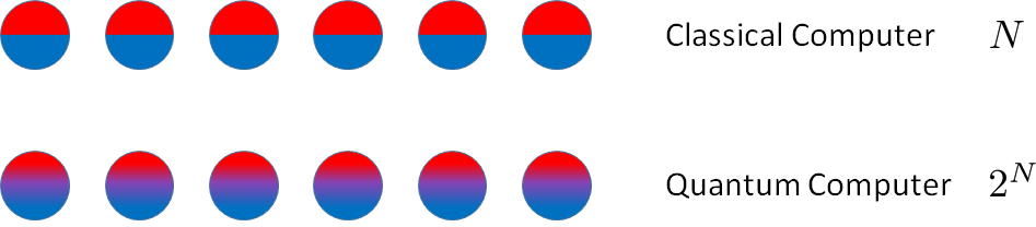
The quantum phenomenon of superposition allows a system to traverse many trajectories in parallel, and determine its state by their coherent sum. In some sense, this coherent sum amounts to massive quantum parallelism. It should not, however, be confused with classical parallel computing, where many “bits” are used instead of one “qubit” in a superposition state.²

Pachos’ book³ also has a clear explanation on this topic.

Quantum Computations

Procedures of Quantum Computation

The over-simplification of Quantum Computation is as such:

• Initialization of the system in a given state $\ket{\psi_i}$. This system can be a many-body system, thus entanglements amongst subsystems are possible. The presence of entanglement dramatically increases the dimension of the encoding space.
• Manipulation of the system. Usually done by letting the system evolve unitarily according to a certain Hamiltonian $H$, then according to the Schrödinger Equation, $\ket{\psi}=U(t) \ket{\psi_i}$, where $\tfrac{\d U}{\d t} = iH(t)U(t)/\hbar$. $U$ is often referred to as the quantum gate.
• Measurement of the system. Such measurement will break any superposition of the system. The system will give a certain outcome for each measurement.

Setup of Toy Quantum Computation: Qubits, Gates

As is described in the last section, qubits are considered as a two-level system throughout this series of posts unless otherwise specified. A typical two-level system is an electron in an external magnetic field. Such electron has two energy levels, namely spin up and spin down.

I am going to use a $\tfrac{1}{2}$-spin particle such as an electron as a qubit to make the discussion more intuitive. Note that experimentally, that’s not how it’s done; it is way more complicated than just manipulating an electron (e.g. IBM). Yet, we can use such “thought experiment” to gain some insights on quantum computers.

Initialization

The states can be conveniently initialized by a measurement. More importantly, an entangled state can be prepared by a measurement of $H\propto \vec S_1 \cdot \vec S_2$.

Manipulation

As quantum evolutions are described by unitary matrices, quantum gates between $n$ qubits are elements of the unitary group $U(2n)$. For example, one qubit gates include the Pauli matrices

\[\sigma_x = \begin{pmatrix} 0& 1\\ 1 & 0\end{pmatrix}, \quad \sigma_y = \begin{pmatrix} 0& -\imath \\ \imath & 0\end{pmatrix}, \quad \sigma_z = \begin{pmatrix} 1& 0\\ 0 & -1\end{pmatrix}.\]

Where $\sigma_x$ is known as the classical $NOT$ gate that changes the input $0$ or $1$ to the output $1$ or $0 $, respectively.

\[\sigma_x \ket{0} = \begin{pmatrix} 0& 1\\ 1 & 0\end{pmatrix} \cdot \begin{pmatrix}1\\0\end{pmatrix} = \begin{pmatrix}0\\1\end{pmatrix} = \ket{1} \\ \sigma_x \ket{1} = \begin{pmatrix} 0& 1\\ 1 & 0\end{pmatrix} \cdot \begin{pmatrix}0\\1\end{pmatrix} = \begin{pmatrix}1\\0\end{pmatrix} = \ket{0}\]

By adjusting the orientations of the magnetic field, since $\sigma_x,\sigma_y,\sigma_z$ are the generators of this Lie group, any unitary matrix can be implemented as $\sigma_{\vec d} = d_1\sigma_x+d_2\sigma_y+d_3\sigma_z$, where $\vec d$ is a unitary vector along the direction of the magnetic field. For example, The Hadamard gate is

\[H = \frac{1}{\sqrt 2}\begin{pmatrix} 1& 1\\ 1 & -1\end{pmatrix} = \sigma_{\scriptsize (\tfrac{1}{\sqrt 2}, \tfrac{1}{\sqrt 2},0)}.\]

To create entanglement between two qubits we need to introduce two qubit quantum gates. An important class of two qubit gates is the controlled gates, $CU$. These gates treat one qubit as the controller and the other one as the target. The action of $CU$ is to leave the target qubit unaffected when the control is in state $\ket0$ and to apply the unitary matrix $U$ on the target qubit when the control is in state $\ket1$. One of them being $CNOT$

\[CNOT = \begin{pmatrix}1 & 0 & 0 & 0 \\ 0 & 1 & 0 & 0 \\ 0 & 0 & 0 & 1\\ 0 & 0 & 1 & 0 \end{pmatrix}.\]

Measurement

The measurement is described by the projection matrix

\[P=\ket{\psi}\bra{\psi}\]

while projections of a many-qubit state onto an entangled two-qubit state can also be considered.

Example of Quantum Circuit

See Grover’s Algorithm, or a documentation for Grover’s Algorithm from IBM. The famous Shor’s algorithm can also be found at IBM’s documentation.

Acknowledgement

This series is made possible by Dr. Emil Prodan’s kind mentorship.

---