---

\[\newcommand{\bra}[1]{\left\langle{#1}\right\vert } \newcommand{\ket}[1]{\left\vert {#1}\right\rangle} \newcommand{\braket}[2]{\left\langle {#1} \, \middle\vert \,{#2} \right\rangle } \newcommand{\uvec}{\hat} \newcommand{\dfdas}{:=} \newcommand{\Eqn}[1]{\text{Eqn. (}\ref{#1}\text{)}} \newcommand{\set}[1]{\left\lbrace {#1}\right\rbrace} \newcommand{\vac}{ {1\!\!1}} \newcommand{\la}{\mathfrak} \newcommand{\anti}{\overline} \newcommand{\Id}{\mathbb I} \newcommand{\e}{\mathrm{e}} \notag \require{cancel}\]

Properties of Ising Anyons

This post mostly follows Pachos’s book of introduction to topological quantum computation.

Fusion Channels

There are three elements in the Ising anyons model. A fermion denoted as $\psi$, an anyon denoted as $\sigma$, and vacuum $\vac$. The fusion rules are

\[\begin{array}{cccccc} \vac \times \vac =& \vac & \vac \times \psi =& \psi & \vac \times \sigma =& \sigma \\ & & \psi\times \psi =& \vac & \psi\times \sigma =& \sigma \\ & & & & \sigma\times\sigma =& \vac+\psi. \end{array}\]

The physical significance, as well as experimental realization, will not be discussed in this post.

If you write the consecutive fusion result of $\sigma$ anyons, you will have

\[\begin{align*} \sigma \times \sigma \times \sigma &= (\sigma \times \sigma) \times \sigma \\ &=(\vac + \psi)\times \sigma\\ &=\vac \times \sigma + \psi \times \sigma\\ &=\sigma + \sigma \\ & = 2\sigma \end{align*}\]

Where the $2$ does not mean two sigma anyons. It is means that there are two fusion channels or paths, one of them passes through $\vac$ and the other passes through $\psi$. Both of them end up with one $\sigma$ anyon. Thus, $2$ retains the dimension of this fusion space. See below when we actually find the fusion space for $\sigma\times\sigma\times\sigma=2\sigma$ in calculating $F_{\sigma\sigma\sigma}^\sigma$’s elements

$F$-Matrices

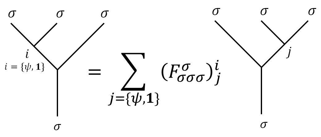
If we list all the possible combinations of fusion tree, the only non-trivial ones are those have $\sigma\times \sigma=\psi+\vac$ as intermediate results. In that case, $a$ and $b$ must be $\sigma$ on the left fusion tree, $b$ and $c$ must be $\sigma$ on the right fusion tree, the total fusion is either $\vac$ with $\sigma$ or $\psi$ with $\sigma$, leaving the $d$ a $\sigma$ anyon.

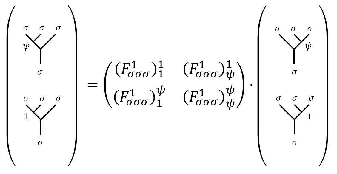
Thus the only non-trivial $F$-matrix is $F_{\sigma\sigma\sigma}^\sigma$, for simplicity, this matrix will be denoted as $F$ when there is no possible confusion. Since there are only two fusion channels, $F$ is a $2\times 2$ matrix, whose indices can only be $\set{\psi,\vac}$.

As expected, since there are only three types of anyons including vacuum, the pentagon equation will be simplified. To calculate the explicit elements of $F_{\sigma\sigma\sigma}^\sigma$, we fill in some of the blanks.

The key is to make sure our target $F_{\sigma\sigma\sigma}^\sigma$ appears somewhere in the edge of the pentagon. But we need to draw multiple Pentagon diagrams to have enough equations to solve for the $F$-matrices.

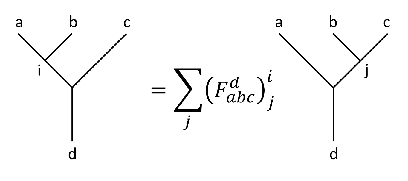
The $F$ matrices is better understood with the following diagram as basis transformation:

With additional “branches” of the fusion tree, we have:

or with irregular elements like the following one.

The inverse is written as

Step 1: First Pentagon

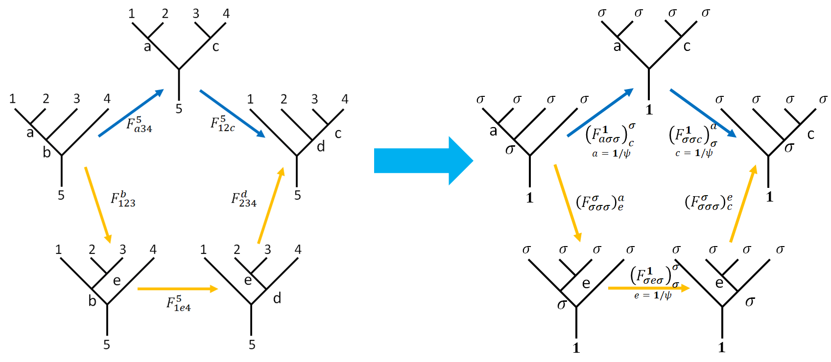
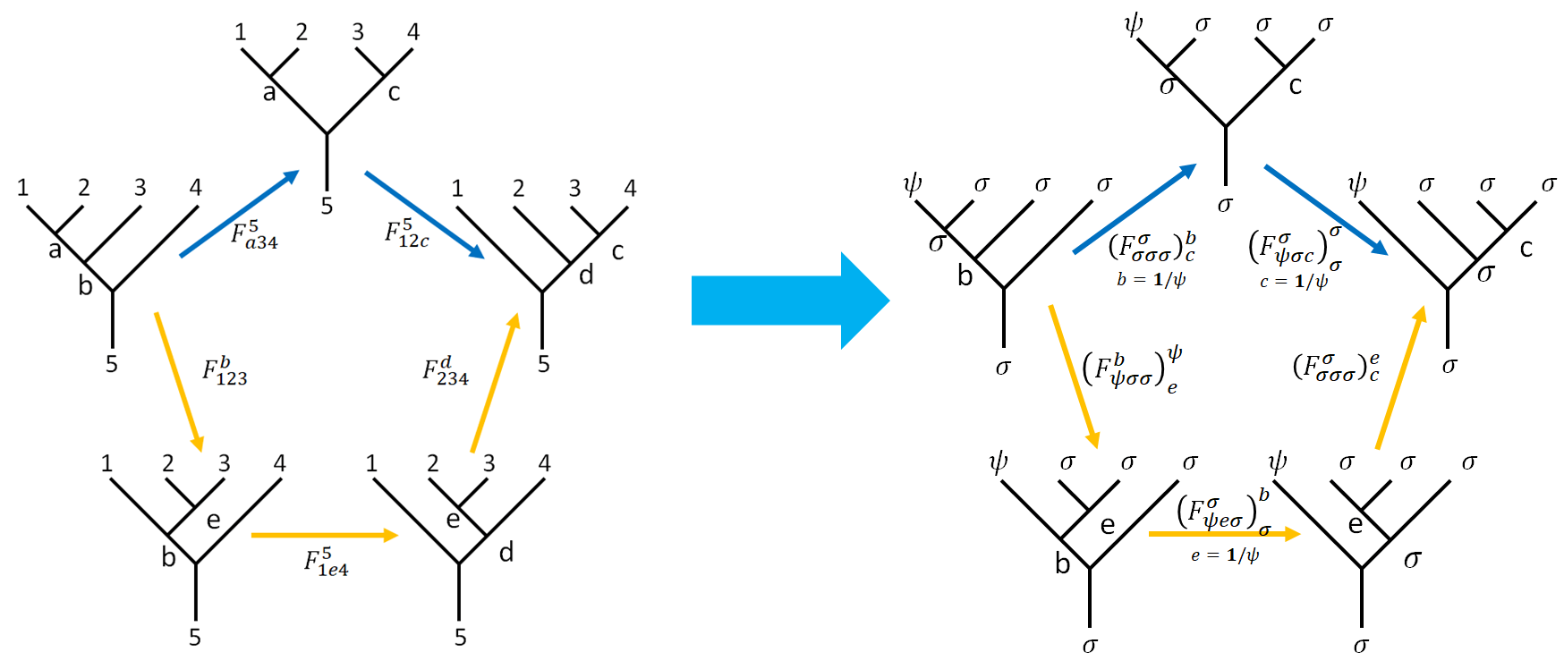
The pentagon equation is written as

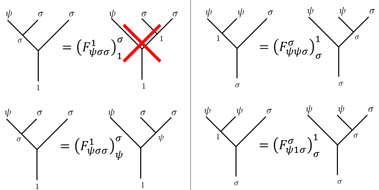
\[\begin{align}\left(F_{a34}^5\right)_c^b \left(F_{12c}^5\right)_d^a & = \sum_e \left(F_{123}^b\right)_e^a \left(F_{1e4}^5\right)_d^b \left(F_{234}^d\right)_c^e \notag\\ &\downarrow \set{1,2,3,4,b,d} =\set{\sigma},\ 5=\vac \notag\\ \left(F_{a\sigma\sigma}^\vac\right)_c^\sigma \left(F_{\sigma\sigma c}^\vac\right)_\sigma ^a & = \sum_e \left(F_{\sigma\sigma\sigma}^\sigma\right)_e^a \left(F_{\sigma e\sigma}^\vac\right)_\sigma^\sigma \left(F_{\sigma\sigma\sigma}^\sigma\right)_c^e \label{penta} \end{align}\]

Apart from $F_{\sigma\sigma\sigma}^\sigma$, all other $F$-matrices are just $\mathbb{C}$-numbers, up to an overall phase factor. This corresponds to a gauge degree of freedom that I will fix to $+1$ (or $-1$, read on to see when it’s $-1$). We are going to find and list the trivial $F$-matrices appeared in $\Eqn{penta}$ so we can use them in the pentagon equation to obtain $F_{\sigma\sigma\sigma}^\sigma$.

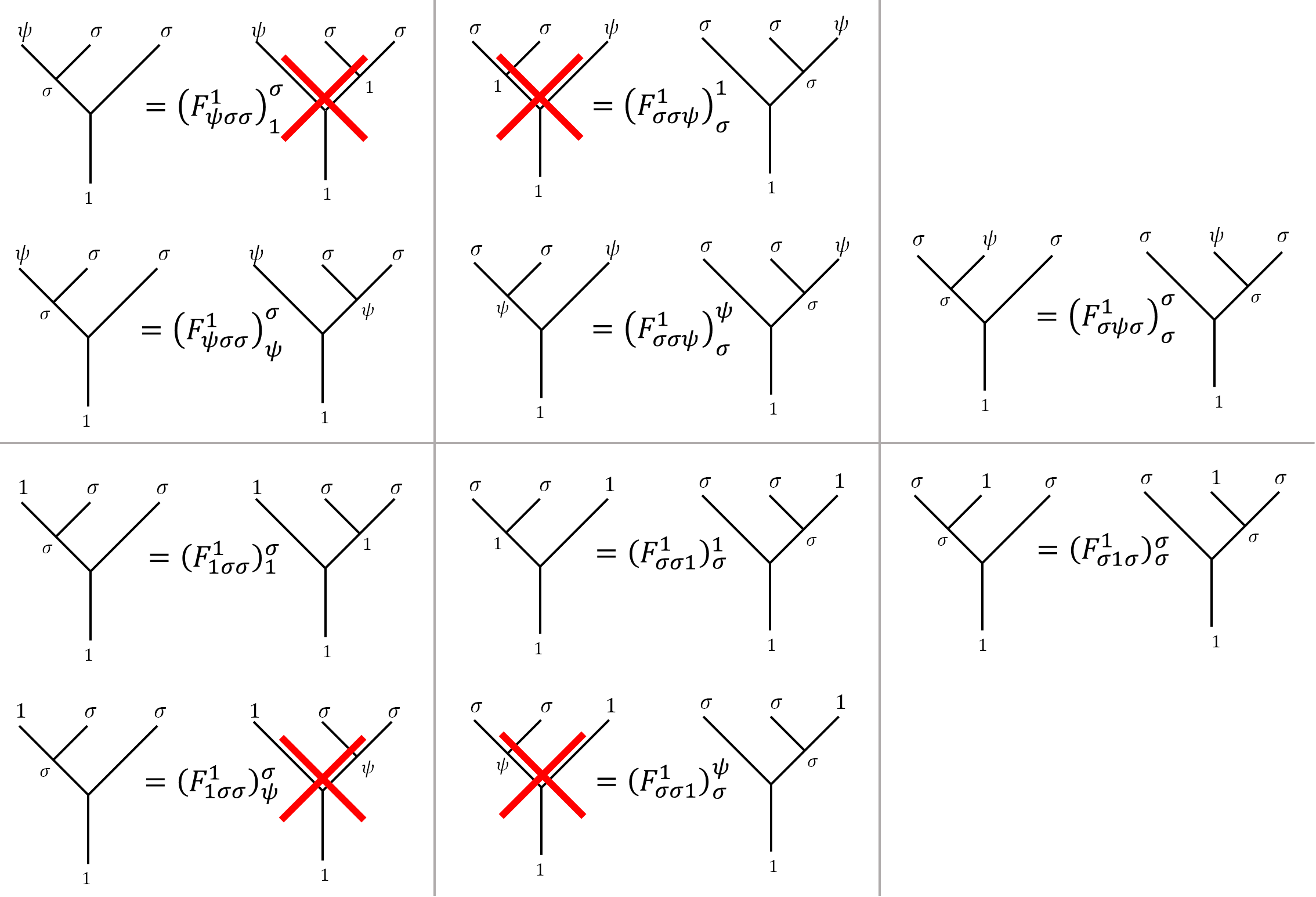
Notice the forbidden fusion tree is marked with a large red cross. $F$-matrices with such trees are just $0$. Substitute corresponding values of $a,c$ into $\left(F _ {a\sigma\sigma}^\vac\right) _ c^\sigma \left(F _ {\sigma\sigma c}^\vac\right) _ \sigma ^a = \sum _ e F _ e^a \left(F _ {\sigma e\sigma}^\vac\right) _ \sigma^\sigma F _ c^e$, we have

	$a =\vac$	$a= \psi$
$c=\vac$	\(\begin{align*}\left(F_{\vac\sigma\sigma}^\vac\right)_\vac^\sigma \left(F_{\sigma\sigma \vac}^\vac\right)_\sigma ^\vac &= \sum_e F_e^a \left(F_{\sigma e\sigma}^\vac\right)_\sigma^\sigma F_c^e\\1\cdot 1=& F_\psi^\vac \left(F_{\sigma \psi\sigma}^\vac\right)_\sigma^\sigma F_\vac^\psi + F_\vac^\vac \left(F_{\sigma \vac\sigma}^\vac\right)_\sigma^\sigma F_\vac^\vac \\1=&F_\psi^\vac \cdot 1 \cdot F_\vac^\psi + F_\vac^\vac \cdot 1 \cdot F_\vac^\vac \\1=& F_\psi^\vac F_\vac^\psi + (F_\vac^\vac)^2\end{align*}\)	\(\begin{align*} \left(F_{\vac\sigma\sigma}^\vac\right)_\psi^\sigma \left(F_{\sigma\sigma \psi}^\vac\right)_\sigma ^\vac &= \sum_e F_e^\vac \left(F_{\sigma e\sigma}^\vac\right)_\sigma^\sigma F_\psi^e\\0\cdot 0 =& F_\psi^\vac \left(F_{\sigma \psi \sigma}^\vac\right)_\sigma^\sigma F_\psi^\psi + F_\vac^\vac \left(F_{\sigma \vac\sigma}^\vac\right)_\sigma^\sigma F_\psi^\vac\\0=&F_\psi^\vac F_\psi^\psi + F_\vac^\vac F_\psi^\vac\end{align*}\)
$c=\psi$	\(\begin{align*}\left(F_{\psi\sigma\sigma}^\vac\right)_\vac^\sigma \left(F_{\sigma\sigma \vac}^\vac\right)_\sigma ^\psi &= \sum_e F_e^\psi \left(F_{\sigma e\sigma}^\vac\right)_\sigma^\sigma F_\vac^e\\0\cdot 0 =& F_\vac^\psi \left(F_{\sigma \vac \sigma}^\vac\right)_\sigma^\sigma F_\vac^\vac + F_\psi^\psi \left(F_{\sigma \psi\sigma}^\vac\right)_\sigma^\sigma F_\vac^\psi\\0=&F_\vac^\psi F_\vac^\vac + F_\psi^\psi F_\vac^\psi\end{align*}\)	\(\begin{align*}\left(F_{\psi\sigma\sigma}^\vac\right)_\psi^\sigma \left(F_{\sigma\sigma \psi}^\vac\right)_\sigma ^\psi & = \sum_e F_e^\psi \left(F_{\sigma e\sigma}^\vac\right)_\sigma^\sigma F_\psi^e\\1\cdot 1=&F_\psi^\psi \left(F_{\sigma \psi\sigma}^\vac\right)_\sigma^\sigma F_\psi^\psi + F_\vac^\psi \left(F_{\sigma \vac\sigma}^\vac\right)_\sigma^\sigma F_\psi^\vac\\1=&F_\psi^\psi \cdot 1\cdot F_\psi^\psi + F_\vac^\psi \cdot 1 \cdot F_\psi^\vac\\1=&(F_\psi^\psi) ^2 + F_\vac^\psi F_\psi^\vac\end{align*}\)

Notice that the above identities are about elements, so the elements are associative. Rearrange and collect the results:

\[\begin{array}{} 1 = F_\psi^\vac \cdot F_\vac^\psi + (F_\vac^\vac)^2 & & 1=F_\psi^\vac \cdot F_\vac^\psi + (F_\vac^\vac)^2 \\ 1 = F_\psi^\vac \cdot F_\vac^\psi + (F_\psi^\psi)^2 & \Rightarrow& \\ 0=F_\psi^\vac(F_\psi^\psi + F_\vac^\vac)& & F_\psi^\psi =- F_\vac^\vac \end{array}\]

As you can see, there are only two independent equations, from diagonal parts of the above table.

Step 2: Second Pentagon

We can draw a second pentagon as below.

This time we are going to find out the two sets of independent equations from $\Eqn{penta2}$ and only list the $F$-matrices appears in those equations.

\[\begin{align}\left(F_{a34}^5\right)_c^b \left(F_{12c}^5\right)_d^a & = \sum_e \left(F_{123}^b\right)_e^a \left(F_{1e4}^5\right)_d^b \left(F_{234}^d\right)_c^e \notag\\ &\downarrow \set{2,3,4,5,a,d} =\set{\sigma},\ 1=\psi \notag\\ \left(F_{\sigma\sigma\sigma}^\sigma\right)_c^b \left(F_{\psi\sigma c}^\sigma\right)_\sigma^\sigma & = \sum_e \left(F_{\psi\sigma\sigma}^b\right)_e^\sigma \left(F_{\psi e\sigma}^\sigma\right)_\sigma^b \left(F_{\sigma\sigma\sigma}^\sigma\right)_c^e \label{penta2}\\ \end{align}\]

The two sets of independent equation can be obtained by setting $b=\vac, c=\vac $ and $b=\vac, c=\psi$. After finding the trivial $F$-matrices associated with the equations,

We have:

\(b=\vac ,\ c=\vac\)

\(b=\vac ,\ c=\psi\)

\(\begin{align*}F_\vac^\vac \left(F_{\psi\sigma \vac}^\sigma\right)_\sigma^\sigma &= \sum_e \left(F_{\psi\sigma\sigma}^\vac\right)_e^\sigma \left(F_{\psi e\sigma}^\sigma\right)_\sigma^\vac F_\vac^e \\F_\vac^\vac \cdot =& \left(F_{\psi\sigma\sigma}^\vac\right)_\psi^\sigma \left(F_{\psi \psi\sigma}^\sigma\right)_\sigma^\vac F_\vac^\psi + \left(F_{\psi\sigma\sigma}^\vac\right)_\vac^\sigma \left(F_{\psi \vac\sigma}^\sigma\right)_\sigma^\vac F_\vac^\vac\\F_\vac^\vac =& 1\cdot1\cdot F_\vac^\psi + 0\cdot 1 \cdot F_\vac^\vac\\F_\vac^\vac=&F_\vac^\psi\end{align*}\)

\(\begin{align*}F_\psi^\vac \left(F_{\psi\sigma \psi}^\sigma\right)_\sigma^\sigma & = \sum_e \left(F_{\psi\sigma\sigma}^\vac\right)_e^\sigma \left(F_{\psi e\sigma}^\vac\right)_\sigma^\vac F_\psi^e \\F_\psi^\vac \cdot ({\color{red}-1})=&\left(F_{\psi\sigma\sigma}^\vac\right)_\vac^\sigma \left(F_{\psi \vac\sigma}^\sigma\right)_\sigma^\vac F_\psi^\vac + \left(F_{\psi\sigma\sigma}^\vac\right)_\psi^\sigma \left(F_{\psi \psi\sigma}^\vac\right)_\sigma^\vac F_\psi^\psi\\-F_\psi^\vac=&0\cdot 1\cdot F_\psi^\vac +1\cdot1\cdot F_\psi^\psi\\-F_\psi^\vac=&F_\psi^\psi\end{align*}\)

where $\left(F_{\psi\sigma \psi}^\sigma\right)_\sigma^\sigma = -1$ is a choice to make $F$-matrix unitary. As the reason for doing so, see About the "Arbitrary Phase Factor".

Step 3: Solve for the $F$-Matrix

So far we have $4$ equations for the elements. Notice the fact that $F$-matrix is unitary does not appear as a constraint but serves as a condition to be satisfied after our choices of gauge (i.e., the arbitrary phase factor).

\[\begin{align*} 1 &=F_\psi^\vac \cdot F_\vac^\psi + (F_\vac^\vac)^2 \\ F_\psi^\psi &=- F_\vac^\vac\\ F_\vac^\vac &= F_\vac^\psi \\ F_\vac^\vac &= - F_\psi^\psi \end{align*}\]

Which we can solve for the elements of $F$ as

\[F= \begin{pmatrix} F_\vac^\vac & F_\psi^\vac \\ F_\psi^\vac & F_\psi^\psi \end{pmatrix} =\pm \frac{1}{\sqrt2} \begin{pmatrix} 1 & 1 \\ 1 & -1 \end{pmatrix}\]

where the $\pm$ is called the Frobenius–Schur indicator (see Pachos).

About the “Arbitrary Phase Factor”

From ¹:

Given a set of fusion rules $N^k_{i,j}$ solving the pentagons turns out to be a difficult task (even with the help of computers). However, certain normalizations can be made to simplify the solutions. If one of the indices of the $F$-matrix $a, b, c$ is the trivial type $\vac$, we may assume $F^{d} _ {a,b,c} = 1$. In the Fibonacci theory, we may also assume $F _ {a,b,c}^\vac = 1$. There are many pentagons even for the Fibonacci theory depending on the four anyons to be fused and their total charges: a priori $2^5 = 32$.

While in Pachos’ book, the explanation for some elements is set to $1$ was simply “otherwise the $F$-matrix wouldn’t be unitary”. I suspect the justification is or (superficially) a direct result from brute force calculation, or may be related to the category theory. For now, I will stop digging deeper and be content with what I have.

$R$-matrices

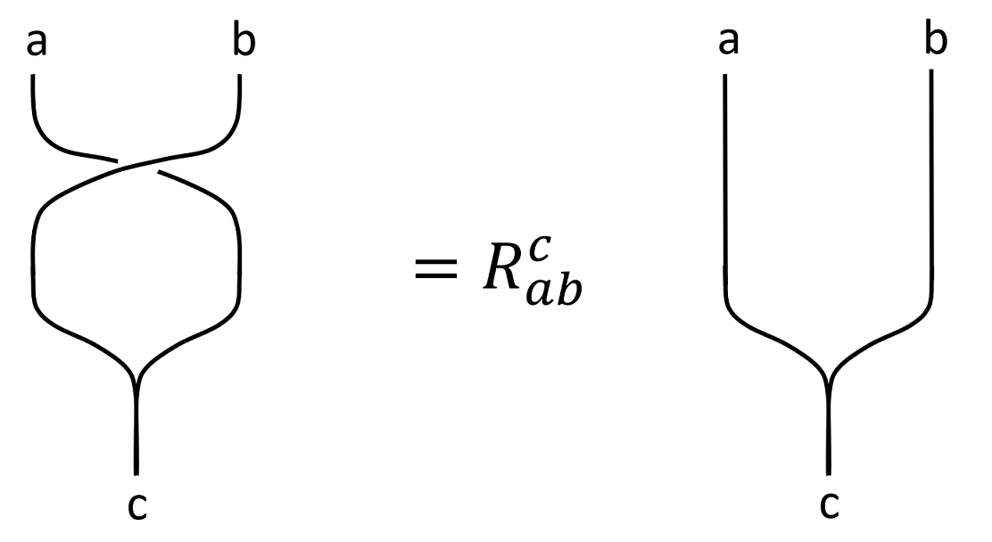
Recall the $R$-matrix as above. The $R$ matrix is understood as a basis transformation of fusion trees like the following.

With all the $F$ matrices figured out, $R$-matrix is easy to calculate. The $R$-matrix is trivial if either $a$ or $b$ is vacuum. Since moving around a particle would not result in any topological phase.

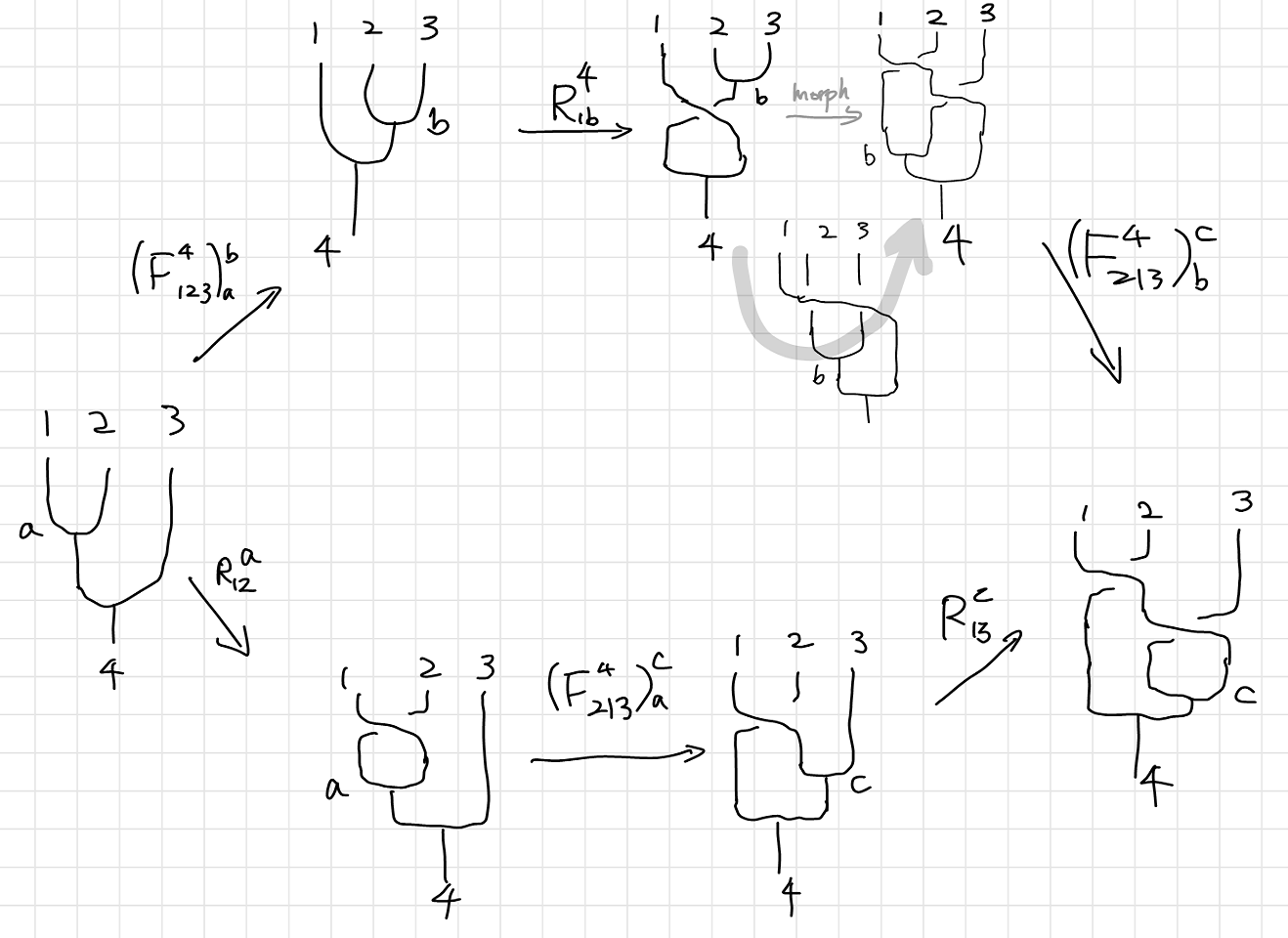
\(\begin{array}{} \sum_b \left(F_{312}^4\right)_b^a R_{3b}^4 \left(F_{123}^4 \right)_c^b = R_{13}^a \left(F_{132}^4\right)_c^a R_{23}^c & \text{Simon's version.}\\ \sum_b \left(F_{231}^4\right)_b^c R_{1b}^4 \left(F_{123}^4 \right)_a^b = R_{13}^c \left(F_{213}^{4}\right)_a^c R_{12}^a &\text{Pachos' version}. \end{array}\)

I will chose to use Simon’s version. Pachos’ version is discussed in his book in detail. Using $\set{1,2,3,4}=\set{\sigma}$, we have for $b=\vac,\psi$:

\[\sum_b \left(F_{\sigma\sigma\sigma}^\sigma\right)_b^a R_{\sigma b}^\sigma \left(F_{\sigma\sigma\sigma}^\sigma \right)_c^b = R_{\sigma\sigma}^a \left(F_{\sigma\sigma\sigma}^\sigma\right)_c^a R_{\sigma\sigma}^c\\ \Rightarrow F_\vac^a R_{\sigma \vac}^\sigma F_c^\vac + F_\psi^a R_{\sigma \psi}^\sigma F_c^\psi = R_{\sigma\sigma}^a F_c^a R_{\sigma\sigma}^c\]

Now substitute the corresponding $a$ and $c$,

	\(a=\vac\)	\(a=\psi\)
\(c=\vac\)	\(\begin{align}F_\vac^\vac R_{\sigma \vac}^\sigma F_\vac^\vac + F_\psi^\vac R_{\sigma \psi}^\sigma F_\vac^\psi &= R_{\sigma\sigma}^\vac F_\vac^\vac R_{\sigma\sigma}^\vac\notag\\\frac{1}{\sqrt2}( R_{\sigma \vac}^\sigma + R_{\sigma \psi}^\sigma) &= R_{\sigma\sigma}^\vac R_{\sigma\sigma}^\vac\label{avaccvac}\end{align}\)	\(\begin{align}F_\vac^\psi R_{\sigma \vac}^\sigma F_\vac^\vac + F_\psi^\psi R_{\sigma \psi}^\sigma F_\vac^\psi &= R_{\sigma\sigma}^\psi F_\vac^\psi R_{\sigma\sigma}^\vac\notag\\ \frac{1}{\sqrt2}(R_{\sigma \vac}^\sigma - R_{\sigma \psi}^\sigma) &= R_{\sigma\sigma}^\psi R_{\sigma\sigma}^\vac\label{apsicvac} \end{align}\)
\(c=\psi\)	\(\begin{align}F_\vac^\vac R_{\sigma \vac}^\sigma F_\psi^\vac + F_\psi^\vac R_{\sigma \psi}^\sigma F_\psi^\psi &= R_{\sigma\sigma}^\vac F_\psi^\vac R_{\sigma\sigma}^\psi\notag\\\frac{1}{\sqrt2}(R_{\sigma \vac}^\sigma - R_{\sigma \psi}^\sigma ) &= R_{\sigma\sigma}^\vac R_{\sigma\sigma}^\psi\label{avaccpsi}\end{align}\)	\(\begin{align}F_\vac^\psi R_{\sigma \vac}^\sigma F_\psi^\vac + F_\psi^\psi R_{\sigma \psi}^\sigma F_\psi^\psi &= R_{\sigma\sigma}^\psi F_\psi^\psi R_{\sigma\sigma}^\psi\notag\\\frac{1}{\sqrt2}( R_{\sigma \vac}^\sigma + R_{\sigma \psi}^\sigma )&= -R_{\sigma\sigma}^\psi R_{\sigma\sigma}^\psi\label{apsicpsi}\end{align}\)

The equations are the same with Pachos version of the hexagon. Notice that there only three independent equations, with an additional condition that circling an anyon around vacuum is trivial, $R_{\sigma\vac}^\sigma=1$.

$\Eqn{avaccvac}$ and $\Eqn{apsicpsi}$ implies that $R_{\sigma\sigma}^1=\pm \imath R_{\sigma\sigma}^\psi$. Adding $\Eqn{apsicvac}$ and $\Eqn{apsicpsi}$ gives $\sqrt 2=(1\pm \imath)(R_{\sigma\sigma}^1)^2$.

Finally, we have the solutions:

\[R_{\sigma\vac}^\sigma=1 \quad \text{as a given trivial matrix}\\ R_{\sigma\psi}^{\sigma} = \imath\\ R_{\sigma\sigma}^\psi= \pm \e^{\tfrac{3\pi}{8}\imath} , R_{\sigma\sigma}^\vac= \pm \imath \e^{\tfrac{3\pi}{8}\imath}\]

Where the overall phase is a choice of the combinations of different signs.

The $R_{\sigma\sigma}$ is considered a matrix as

\[R_{\sigma\sigma} = \begin{pmatrix}R_{\sigma\sigma}^\vac &0\\0&R_{\sigma\sigma}^\psi\end{pmatrix}\]

Computation with Ising Anyons

Encoding Single Qubit

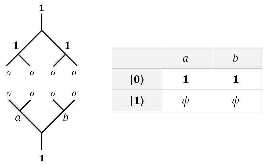
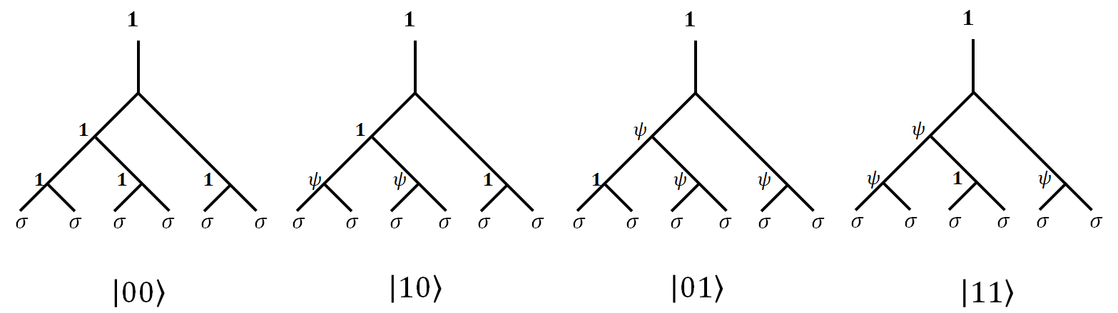
As is described before, since fusion is equivalent to a measurement, the only way to achieve superposition is to have an “incomplete measurement”. For $4$ anyons, a certain total fusion result (called a sector) has two intermediate channels. In our case, we will always pull our $\sigma$ anyons pairwise form the vacuum, and fusion them back into the vacuum.

The upside-down fusion tree symbolizes that these anyons are pulled from the vacuum.

Encoding Two Q-Bits

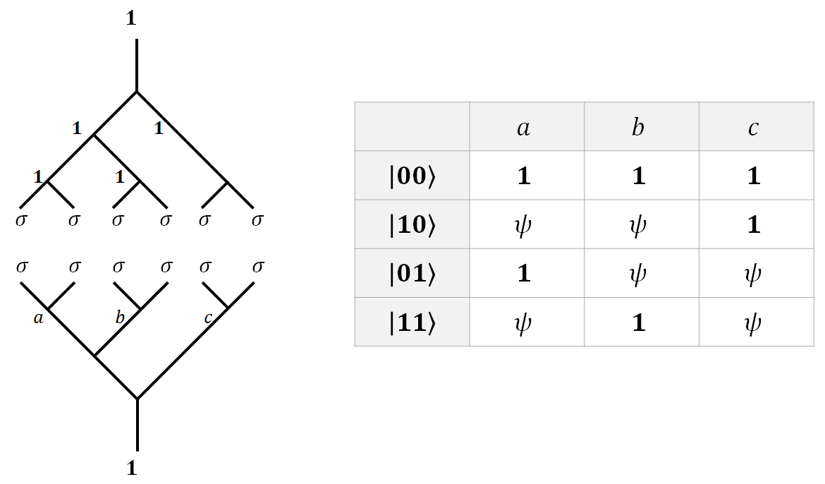
The same can be done for $2$ Qubits. $6$ anyons can encode two qubits. Following the same pattern, $2N$ anyons have $2^{N-1}$ intermediate fusion channels, and can thus encode $N-1$ qubits. The upside-down fusion tree symbolizes that these anyons are pulled from the vacuum.

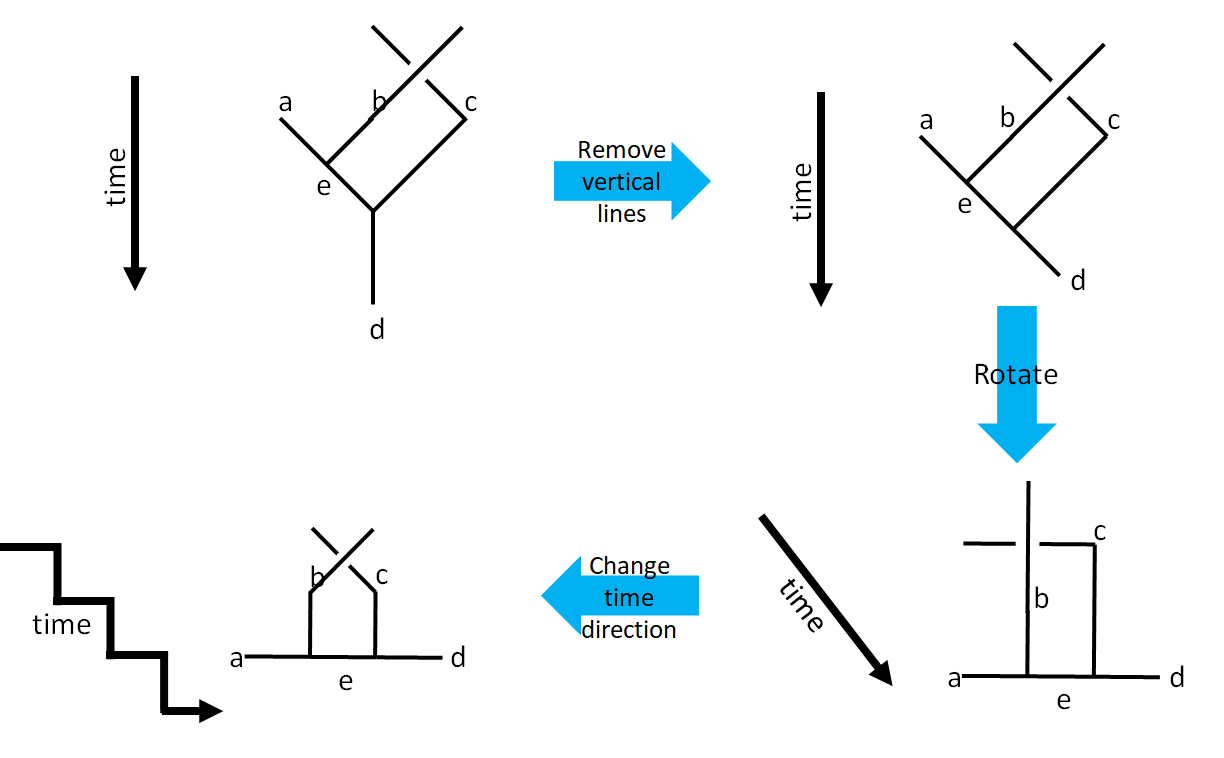
As you can imagine, with the increase in the number of qubits, the fusion tree will become considerably larger and harder to draw. A new type of fusion diagram came into existence just to save some space. The idea depicted as below.

Encoding $n$-qubits

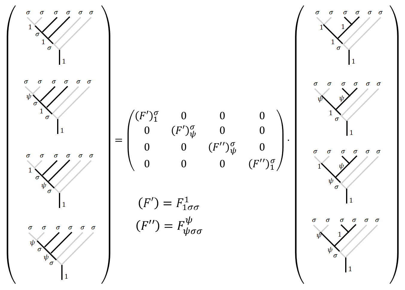
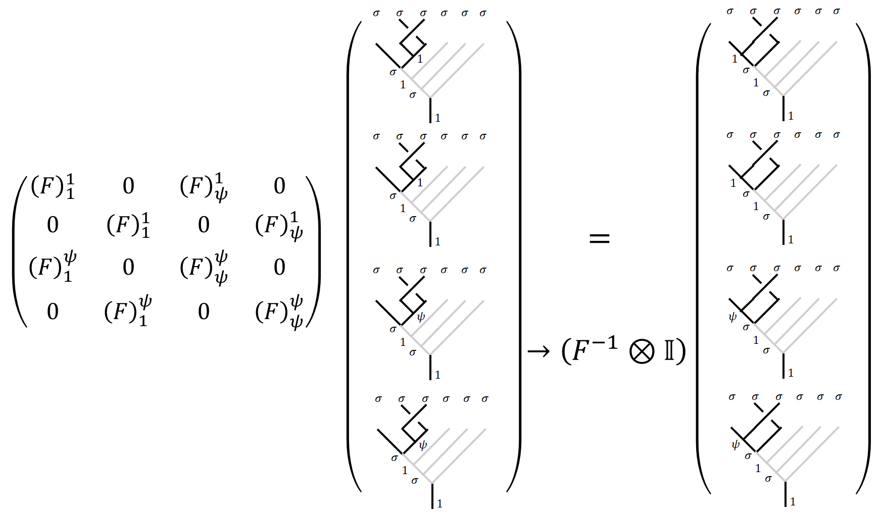
Let’s consider $n$ pairs of $\sigma$ anyons fusing together to $\vac$. Two fusion trees are of particular interest to us. The first one is the canonical fusion tree, the other is the pairwise fusion tree. It’s easy to draw a canonical fusion tree horizontally like the one below, and the pair-wise fusion tree is the one more visually intuitive to encode qubit with. Since the fusion result is irrelevant to the order of fusion, $a_i$ on the canonical tree is in one-to-one correspondence to the pairwise tree. Since $a_i$ is always the fusion result of $2i$ $\sigma$ anyons. Thus the $F$-matrices between these two fusion trees are trivial, for $a_i\neq \sigma$.

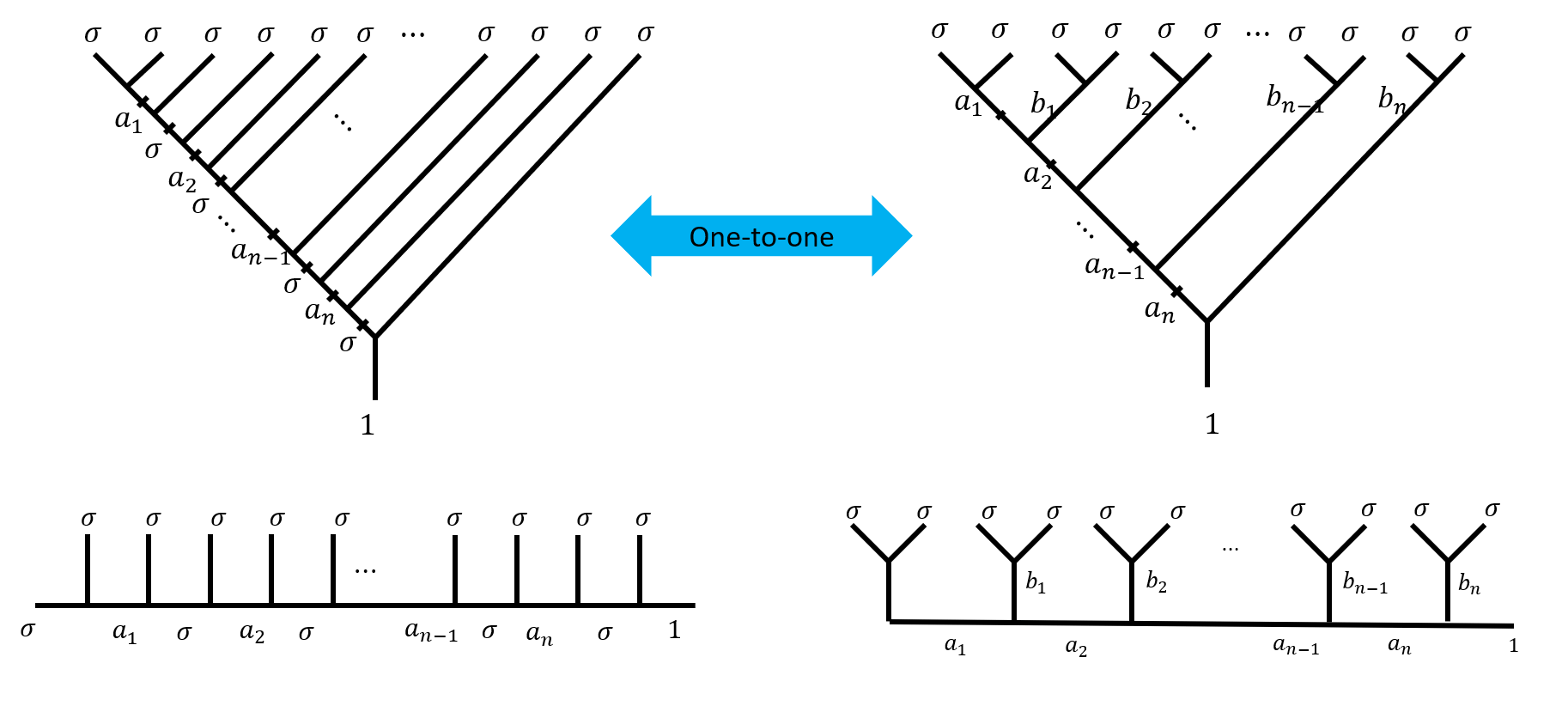
Namely, there is a one-to-one correspondence between the canonical tree and the pairwise tree. This proposition is also evident if you consider that these trees have exactly the same degrees of freedom. So if the pairwise tree can be used to encode qubits, so can the canonical tree. Instead of using $\set{a_1,b_1,b_2,b_3,\cdots,b_n}$ to encode qubits, we can use $\set{a_1,a_2,a_3,\cdots,a_n}$.

Although there are $n+1$ elements in $\set{a_1,b_1,b_2,b_3,\cdots,b_n}$, and only $n$ elements in $\set{a_1,a_2,a_3,\cdots,a_n}$, they do have the same degrees of freedom. For elements in $\set{a_1,a_2,a_3,\cdots,a_n}$, each one is free to choose from $\set{\vac,\psi}$, resulting in to $2^n$ choices; but for elements in $\set{a_1,b_1,b_2,b_3,\cdots,b_n}$, they have to fuse into $\vac$ so there is one additional constrain on them (for example, you can not have odd number of $\psi$), hence there is only $2^{(n+1)-1}$ choices, which is the same as elements in $\set{a_1,a_2,a_3,\cdots,a_n}$.

Initialization

The initialization is then pulling different intermediate anyons from the vacuum. What is the physical process that determines whether a pair of $\sigma$ anyons or a pair of $\psi$ anyons are pulled from the vacuum? As an oversimplification, we can slowly turn on the defects so some excitations as anyons are introduced. Such appearance of anyons can be regarded as “pulling from the vacuum”. In the case of Ising anyons, the building block is $\sigma$ anyon. By introducing defects, $\sigma$ anyons emerge. We can bring the $\sigma$ anyons together pair-wise to see if they behave like a $\psi$ or $\vac$. After such operation, we separate the anyons pair-wise as if they were pulled form $\psi$ or $\vac$. I will leave a detailed answer to the question to a case study of physical realization of such a system in later posts.

For now, we will just concern ourselves with the fact that we can control what to be pulled from the vacuum. As such, $N$ qubits can be prepared.

First Attempt to a Quantum Gate

You might ask that if two anyons are created pairwise from the vacuum, how can they possibly fuse into $\psi$. That is achieved through Braiding to these anyons. In other words, two pairs of $\sigma$ anyons pulled from vacuum respectively can be regrouped pair-wisely and fused. Such intermediate fusion does not necessarily result in $\vac$ since the only constraint is the total fusion to be $\vac$.

So how exactly are we going to arrange our combination of $F$ and $R$ moves, such that it could give us a quantum gate on a qubit? Well, $R$ moves won’t be of much use. If you braid two anyons which originally fuse to $c$, then they will continue fuse to $c$, due to the conservation of topological charges.

Hence, to make the magic happen, as we said before, we need to regroup and then fuse the anyons, like the upper two fusion trees.

In the following calculations, we have chosen the gauge as

\[\begin{array}{cc} F=F_{\sigma\sigma\sigma}^\sigma=\frac{1}{\sqrt2}\begin{pmatrix}1 & 1 \\1 & -1 \end{pmatrix} &\quad R= R_{\sigma\sigma}=\e^{-\tfrac{\pi}{8}\imath}\begin{pmatrix}1 &0\\0&\imath\end{pmatrix}, \\ F^{-1}=\frac{1}{\sqrt2}\begin{pmatrix}1 & 1 \\1 & -1 \end{pmatrix}=F &\quad R^{-1}= \e^{\tfrac{\pi}{8}\imath}\begin{pmatrix}1 &0\\0&-\imath\end{pmatrix} \end{array}\]

Such result can also be directly calculated from specific systems. See Section III. B. 2 of ².

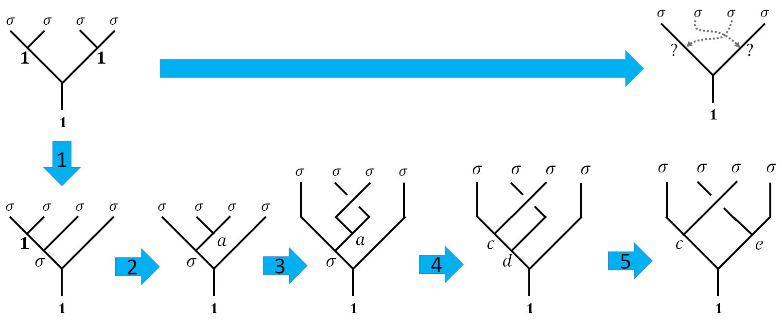
Such action can be achieved through a sequence of $F$ and $R$ moves. We can identify the $R$ and $F$ matrices in the process by writing the following diagrams. Here are the corresponding matrices:

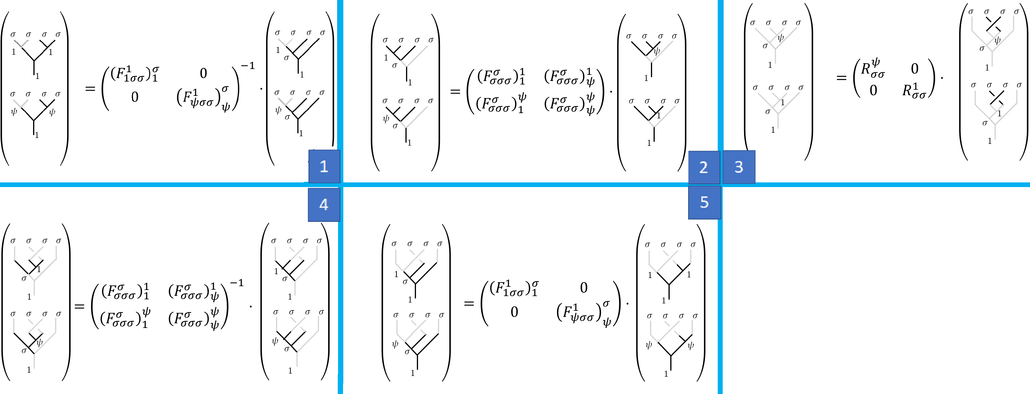
Now let’s calculate the matrix correspond to such fusion, let’s denote the matrix as $B$ for reasons will be clear later.

\[B= \Id^{-1} \cdot F\cdot R\cdot F^{-1}\cdot \Id =\frac{1}{\sqrt 2} \e^{\imath \pi/8} \begin{pmatrix}1&\imath\\\imath&1\end{pmatrix}\]

Where $\Id$ shows again that there is a one-to-one correspondence between the canonical tree and the pairwise tree.

$B$ is conveniently the square root of $\sigma_x=\begin{pmatrix}0&1\newline 1&0\end{pmatrix}$ with an overall phase. Which we can construct by repeating the above result. Alternatively, we can rotate the middle two anyons twice, which numerically

\[B'=\Id^{-1} \cdot F\cdot R^2\cdot F^{-1}\cdot \Id =\Id^{-1} \cdot F\cdot R\cdot \cancel{\left(F^{-1}\cdot \Id\cdot\Id^{-1} \cdot F\right)}\cdot R\cdot F^{-1}\cdot \Id = (B)^2.\]

After so much trouble, we found a single qubit gate $X=\sigma_x$. As you can imagine, if we want to write an $n$-qubit gate, even if $n=2$, writing down all these fusion trees will be very painful.

Alternatively, you can start from one fusion tree and enumerate all the possible moves and see whether the path lead you to your destination. You can see that there are so many diagrams that are marked “undefined”, which are moves that exchange two anyons that are not fused together.

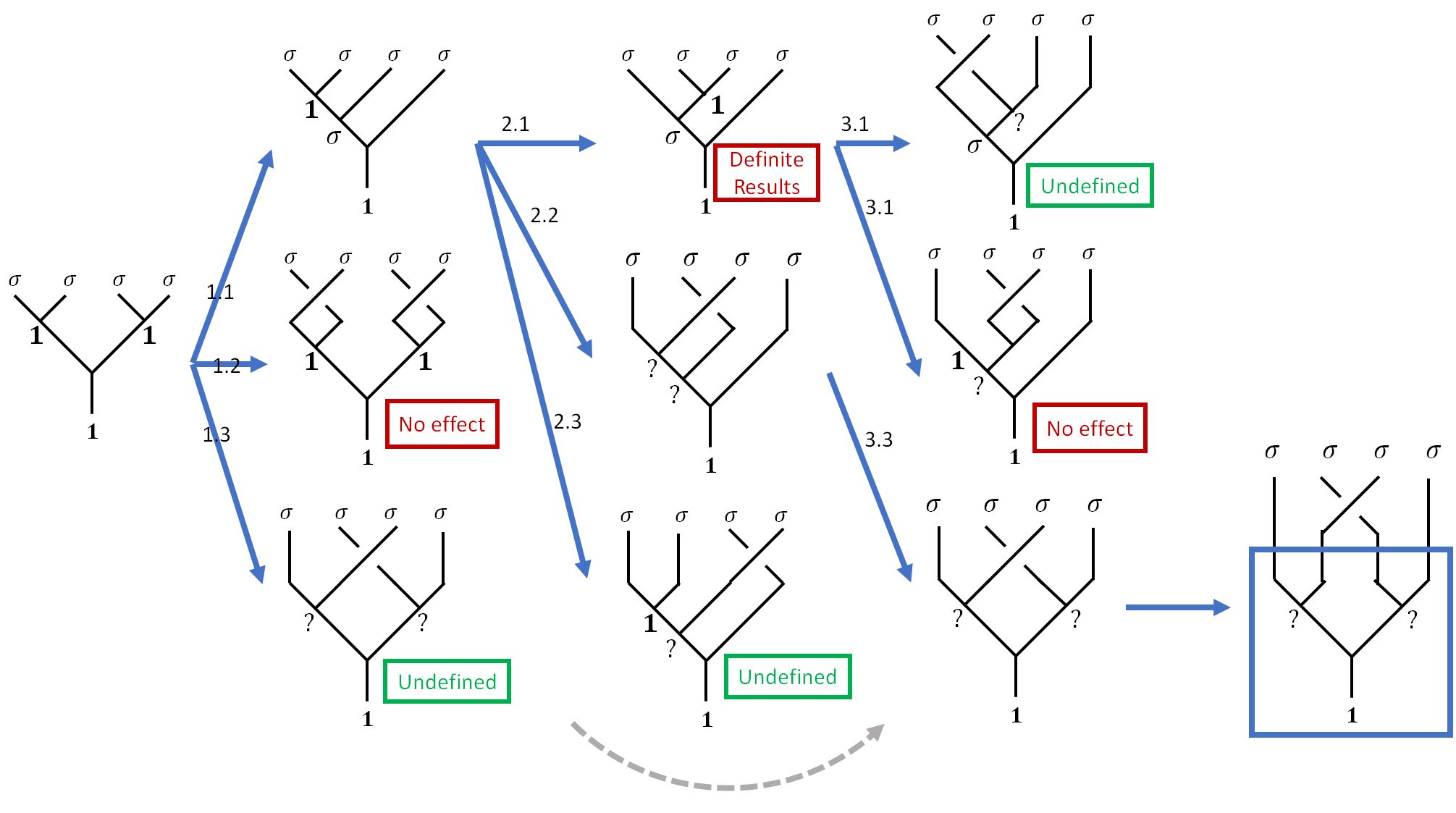
All the trouble is simply because we can not define a matrix that characterizes two non-fusing anyons exchange. How easier our lives will be if only we have such matrix!

Braiding Matrices

Braiding matrix is the savior. What we have got from the last section is the step-by-step construction of a braiding matrix, commonly denoted as $B$. The idea of a braiding matrix is that we can exchange any neighboring anyons without having to worry about whether they are fused together in the next step or not.

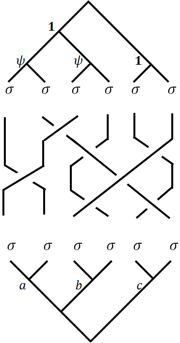
$B$ matrices enable us to consider the moves of anyons in a more direct way. Remember that I introduced figure (c) in the second post of this series.

After pulling anyons from the vacuum and before fusing them together in the end, we can concern ourselves solely on the exchange, depicted below.

Braiding Matrix on Single Qubit

Our mission is then to find out the explicit matrix elements of $B$. The essence of $B$ matrix or a $B$ move is that it exchanges two anyons that are not immediately fused. We can extract the key steps from the braiding procedure as below.

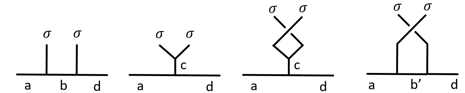
Obviously, an exchange of $(2i-1,2i)$ anyons is not the same as the exchange of $(2i,2i+1)$ anyons on the canonical tree (label start from left to right, starting from $1$). The former exchange is represented by an $R$ matrix, while the later is not a legal $R$ move. The same is true for the pairwise fusion tree. $(2i-1,2i)$ anyon pairs are different from $(2i,2i+1)$ anyon pairs, in that the fusion ingredient and result are distinct.

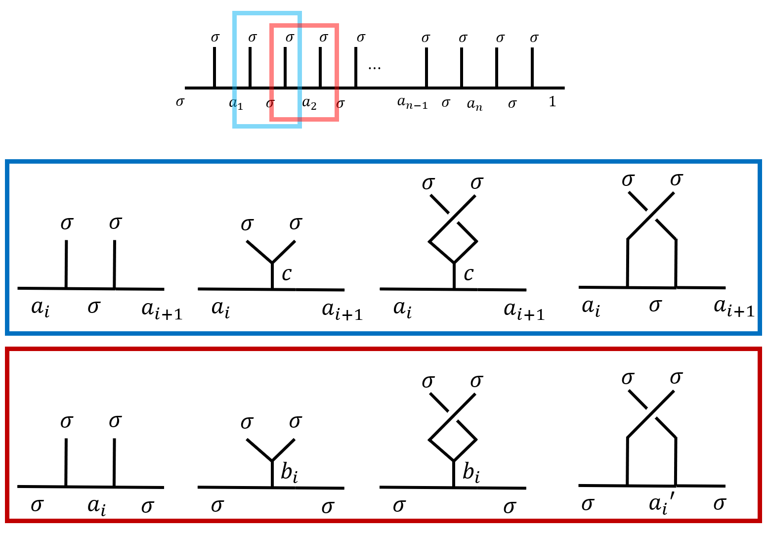
• When $(2i-1,2i)$ are exchanged as is indicated in the blue rectangle, the $F$ matrices are trivial, as $\set{a_i,a_{i+1},c}=\set{\psi,\vac}$. $B_{2i-1,2i}=R_{\sigma\sigma}$.
• When $(2i-1,2i)$ are exchanged as is indicated in the red rectangle, $B_{2i,2i+1}= F\cdot R\cdot F^{-1}$.

Braiding Matrix on two-qubits

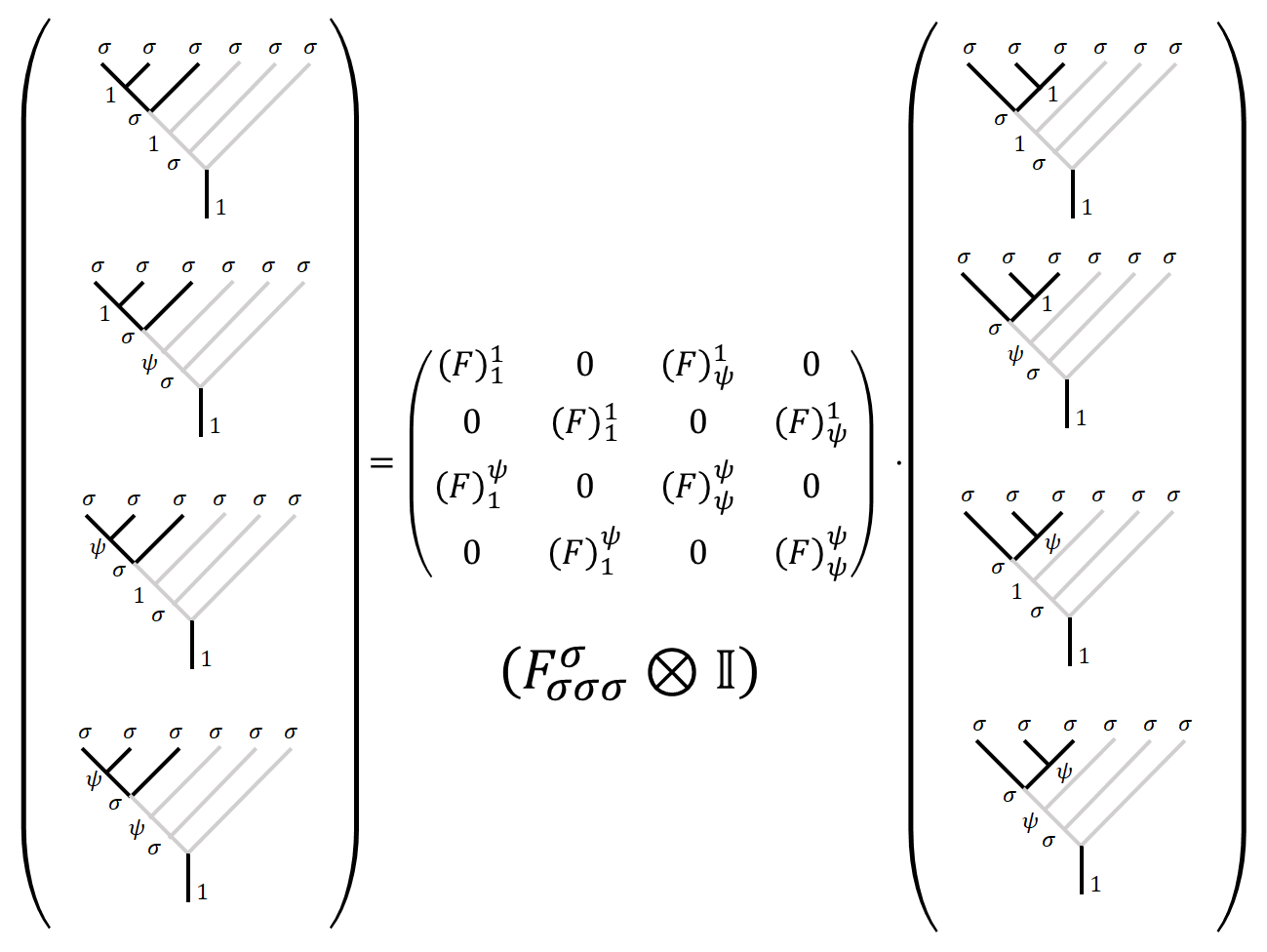
To implement a $B$ matrix on $6$ qubits, we need to write down the $F$ and $R$ matrices on $6$ qubits. Once we have determined $B$ matrices on two qubits fusion space, we will be ready to implement quantum gates, or more specifically, Clifford gates, which generates a large portion of quantum gates.

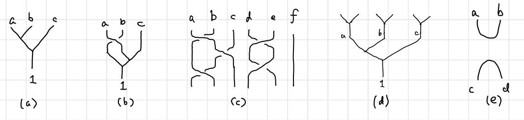
Here are some examples of braiding diagrams with corresponding quantum gates labeled below.

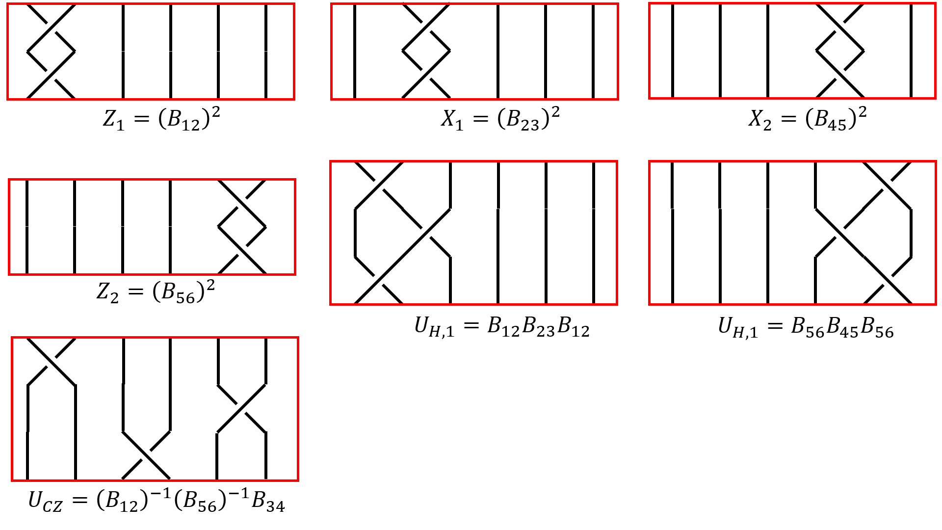
As we have discussed before, the first 6 braiding diagrams are pretty straight forward to calculate, since the $B$ action only act on a sidle qubit and leaves the other invariant, we have $Z$, $X$ and $H$ (Hadamard) gates on qubit $1$ and $2$ as

\[Z_1 = (B_{12}\otimes \Id)^2,\\ Z_2 = (\Id\otimes B_{12})^2,\\ X_1 = (B_{23}\otimes \Id)^2,\\ X_2 = (\Id\otimes B_{45})^2,\\ U_{H,1} = (B_{12}\otimes \Id)\cdot(B_{23}\otimes \Id)\cdot(B_{12}\otimes \Id), \\ U_{H,2} = (B_{56}\otimes \Id)\cdot(B_{45}\otimes \Id)\cdot(B_{56}\otimes \Id).\\\]

But we do not know how to define $B_{34}$ from single-qubit $B$ moves, which is no surprise since $CZ$ gates (or $CPhase$ gates) are fundamentally different from single qubit gates as in it creates entanglement between qubits. To obtain $B_{34}$, we have to write the involved $R$ and $F$ matrices in the $6$-anyon fusion space. Since $3=2i-1,4=2i,(i=2)$ we only need to find out the $R$ matrix.

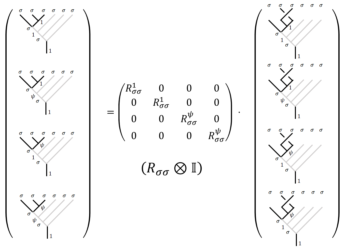
\[B_{34}= R_{34}= \tilde R_{\sigma\sigma}\]

Since our pairwise fusion tree’s basis are $\ket{\vac\vac\vac},\ket{\psi\psi\vac},\ket{\vac\psi\psi},\ket{\psi\vac\psi}$, the $R$ matrices will be non-zero only at diagonal elements, since all the states are distinct (If you are not sure, just draw it yourself, see an example here). Hence we can directly write down the $R$ matrices as

\[\begin{array}{ccccc} R_{12} = \operatorname{diag}(&R^\vac,&R^\psi,&R^\vac,&R^\psi&)\\ R_{34} = \operatorname{diag}(&R^\vac,&R^\psi,&R^\psi,&R^\vac&)\\ R_{56} = \operatorname{diag}(&R^\vac,&R^\vac,&R^\psi,&R^\psi&)\\ \text{Basis:}&\begin{pmatrix}\vac\\\vac\\\vac\end{pmatrix} &\begin{pmatrix}\psi\\\psi\\\vac\end{pmatrix} &\begin{pmatrix}\vac\\\psi\\\psi\end{pmatrix} &\begin{pmatrix}\psi\\\vac\\\psi\end{pmatrix} \end{array}\]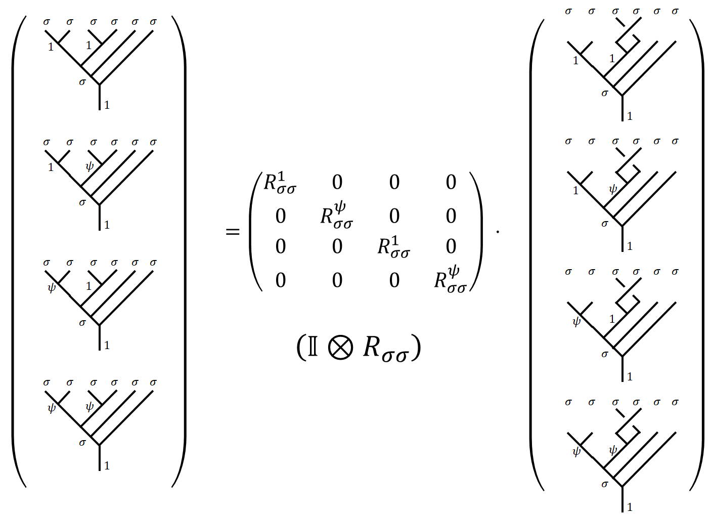

Which gives us the $CZ$ gate we wanted

\[\begin{align*} CZ&=(R_{12})^{-1}(R_{56})^{-1}R_{34} \\ &= \operatorname{diag}(R^\vac,R^\psi,R^\vac,R^\psi)^{-1}\cdot\operatorname{diag}(R^\vac,R^\vac,R^\psi,R^\psi)^{-1}\cdot \operatorname{diag}(R^\vac,R^\psi,R^\psi,R^\vac) \\ & = \operatorname{diag}(1,-\imath,1,-\imath)\cdot\operatorname{diag}(1,1,-\imath,-\imath)\cdot \operatorname{diag}(1,\imath,\imath,1) \\ &=\operatorname{diag}(1,1,1,-1) \end{align*}\]

Clifford Gates v.s. Universal Gates

We have implemented a set of quantum gates $\set{X_1,X_2,Z_1,Z_2,H_1,H_2,CZ}$ which generates the Clifford gates. Sadly that’s the best we can do with Ising anyons, according to³. I think related articles are

• 1.⁴ why MZM can only have Clifford gates,
• 2.⁵ Why do we need gates other than gates from Clifford group.
• 3.⁶ detailed description on Clifford group, points to “Gottesman-Knill theorem” and states “no elementary proof for universality”.

Unfortunately, I do not know much on the topic. The discussion could take on another whole post so hopefully, I can write about that in future posts.

Fusion

To complete our setup for a topological quantum computer, we need to define our fusion operators, which is conveniently defined as projection operators such as $\ket{1}\bra{1}\otimes \Id$. This again reminds us that fusion is just like measurements.

Summary and Outlook

As is stressed before, the only constraint on the entire process of TQC is that we pull everything from the vacuum and return back to vacuum. Sometimes the following diagram is drawn to capture the entire process. The implementation of quantum gates via braiding is a lot like literal “braiding with strands”. Such braiding forms a group named Braid group. Many interesting aspects of the braid group can be understood can be calculated intuitively from the diagrams. What is more interesting is when you connect the open ends of the braiding diagrams: you will get a knot, which is remarkable, for you can imagine that the knot is actually topologically invariant against deformations on which the idea of topological quantum computation is built! Are there any ways to characterize TQC with the topological invariants of knots?

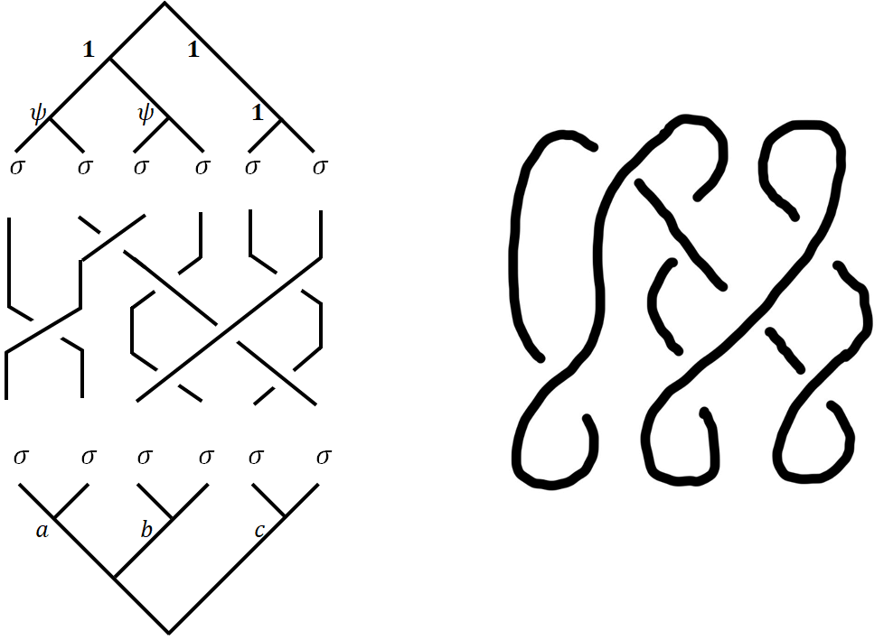
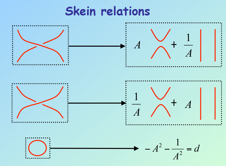
In later posts, we will discuss the Jones polynomials⁷⁸, where you will find some weird equations that motivated me writing this series (picture from ⁷).

Since we are not using QFT/”second quantization”, hence these anyons are still distinguishable, which makes me wonder how the theory goes to make them indistinguishable. This is a long shot and probably won’t be discussed in any posts in the near future.

---