Introduction To Topological Insulator
Posted: September 02, 2019
Edited: October 20, 2019
Status:
Writing
Categories :
Topological-Insulator
Topology
Physics
Tight Binding Model of SSH
This post mainly follows https://arxiv.org/pdf/1509.02295.pdf
Tight Binding Model and Hopping Term
The chapter mainly follows http://www.damtp.cam.ac.uk/user/tong/aqm/aqmtwo.pdf
For a $n$-atom chain, if the electrons are well confined within each atom, we denote the quantum state as $\ket{n}$. These states are considered orthogonal to each other,
\[\braket{n}{m} = \delta_{nm}.\]Here we must make the distinction of an atomic state at site $n$ between a state of an electron at site $n$. These two sets of states confused me for a long time. If you consider $\ket{n}$ as an actual atomic state, they are definitely NOT orthogonal to each other, since the entire concept of hopping and binding (as the name advertised, tight-binding) relies on the “overlap” of these states. But you will further work on the representation of $\ket{n}$ and write the Hamiltonian as a matrix, which means that they ARE orthogonal.
One way to approach this is to assert that a “new set of states were formed when you combine these atoms”, so that $\ket{n}$ are not atomic orbitals but “polymer orbitals” in some sense. However this approach does not answer the question whether or not these states are orthogonal. The other way is to assume that these atoms are separated infinitely far away with each other, but the entire chain has a somewhat finite length, which explains why this a “approximation”. This kind of “occupation states” used in this post is much more easier to understand but has its flaws as well. Electrons do not have a well defined position and you generally cannot say that $\ket{n}$ represent a state of an electron at site $n$.
Beside their mathematical equivalence, the gist of the three approaches are the same: to make such approximation, we need to introduce some artificial constrains that are not quite reasonable. But once again when we judge the theory, we are happy that our surreal approximation gave us a near-realistic result.
The Hilbert space of this system spanned by $\ket{n}$ has dimension $n$. This Hamiltonian dictates that each electron are remained on each atom would be
\[H_0=E_0 \sum_n \ket{n}\bra{n}\]Evidently the solution of the secular equation is
\[H_0\ket{n} = E_0 \ket{n}\]with $\ket{n}$ being the eigenstate and $E_0$ the eigenvalue.
To have a more interesting Hamiltonian that describes electrons “hopping” or tunneling from one site to another, we need extra terms in the Hamiltonian. As the state is governed by the Schrodinger Equation,
\[\ket{\psi (t) } = \emath^{-\imath H t / \hbar } \ket{ \psi(0)} =\left(1-\frac{\imath }{\hbar} H t + \mathcal O(t^2)\right)\ket{ \psi(0)}\]we require that the first order term ($\frac{\imath }{\hbar} H t \ket{\psi(0)}$) has the component on neighboring sites,
\[\bra{n\pm 1}H\ket{n} = t \neq 0\]but not next-nearest or further neighboring sites
\[\bra{n\pm k}H \ket{n} = 0.\]We can write our Hamiltonian as
\[H= \sum_n E_0\ket{n}\bra{n} + t\big(\ket{n+1}\bra{n} + \ket{n}\bra{n+1}\big)\]If we start from a localized state $\ket{n}$, it will spread (or hop) over the chain over time. If we write this Hamiltonian in the basis of $\ket{n}$, we will have a matrix whose eigensystems are readily solved. The magnitude of the hopping parameter $t$ determine how strong the inter-atomic interaction are. Namely, how easily can electron hop from one site to another.


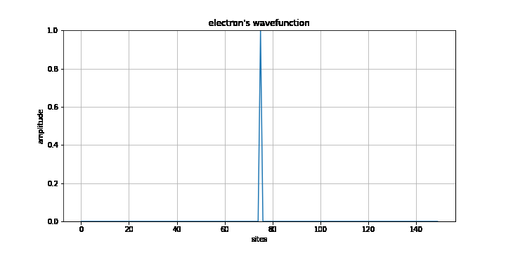
Code
import matplotlib
import matplotlib.pyplot as plt
import numpy as np
import imageio
from scipy.linalg import expm
#
steps = 100
dm = 150
E_0 = 0.
t=0.1
site = int(dm/2)
#
H=[ [0 for i in range(dm)] for j in range(dm) ]
for i in range(dm):
    for j in range(dm):
        if i==j:
            H[i][j]=E_0
        if abs(i-j)==1:
            H[i][j]=t
#
psi_0 = [0 for i in range(dm)]
psi_0[site]=1
#
H= np.array(H)
psi_0 = np.array(psi_0)
psi_o = psi_0
psi_t = [psi_0]
#
for i in range(0,50*steps):
    psi_o = np.matmul(expm(-1j*H/steps),psi_o)
    psi_t.append(np.absolute(psi_o))
#
def plot_for_offset(t):
    fig, ax = plt.subplots(figsize=(10,5))
    ax.plot(psi_t[t])
    ax.grid()
    ax.set(xlabel='sites', ylabel='amplitude',
           title='electron\'s wavefunction')
    ax.set_ylim(0, 1)
#
    fig.canvas.draw()
    image = np.frombuffer(fig.canvas.tostring_rgb(), dtype='uint8')
    image  = image.reshape(fig.canvas.get_width_height()[::-1] + (3,))
    return image
#
kwargs_write = {'fps':1.0, 'quantizer':'nq'}
imageio.mimsave('./powers.gif', [plot_for_offset(20*i) for i in range(250)], fps=40)
Band Structure of Hopping Hamiltonian
The eigenstate of the interesting Hamiltonian can be solved as follow. We expand a state according to the basis set ${\ket{n}}$.
\[\ket{\psi}=\sum_m \psi_m \ket{m}\]Substituting that into the Schrodinger equation, we have
\[\begin{align} H\ket{\psi} &= E\ket{\psi}\\ \sum_n E_0\ket{n}\bra{n} + t\big(\ket{n+1}\bra{n} + \ket{n}\bra{n+1}\big) \sum_m \psi_m\ket{m}&=E\sum_m \psi_m\ket{m} \\ \sum_m\sum_n E_0\psi_m \delta_{mn} \ket{n} + \sum_m \sum_nt\psi_m\ket{n+1}\delta_{mn}+ \sum_m\sum_nt\psi_{m}\ket{n}\delta_{n+1,m} &=\sum_m E \psi_m\ket{m} \\ \sum_m E_0\psi_m\ket{m}+\sum_m t\psi_{m}\ket{m+1}+\sum_m t\psi_{m}\ket{m-1}&=\sum_m E \psi_m\ket{m} \end{align}\]Multiply on both side to the right $\ket n$, we have
\[E_0\psi_n +t(\psi_{n-1}+\psi_{n+1}) = E\psi_n\]Under periodic boundary condition, this set of equations are solved by taking $\psi_n=\emath^{\imath k n a}/\sqrt{N}$, and we see immediately that
\[E(k)= E_0-2t\cos(ka)\]The above conclusion can be generalized to next-nearest hopping and higher, as the equation is readily modified to
\[E_0\psi_n +t_1(\psi_{n-1}+\psi_{n+1})+ t_2(\psi_{n-2}+\psi_{n+2})= E\psi_n\]or if we write $E_0$ as $2t_0$, we have
\[\sum_{i=-h}^{h} t_i\psi_{n+i}=E \psi_n\]where $h$ runs through all hopping atoms. The solution is obtained by taking $\psi_n=\emath^{\imath k n a}/\sqrt{N}$, would be
\[E(k)=\sum_{i=0}^h 2t_i \cos(iak)\]Tight Binding Model in Momentum Space
If we impose a Fourier transformation to our Hamiltonian (with translation invariance), we have the Hamiltonian in the momentum space. To do that, first we identify the momentum eigen states, as
\[\ket{k} = \tfrac{1}{\sqrt N}\sum_m \emath^{\imath ma k} \ket{m}\]And we have for the hopping Hamiltonian,
\[\begin{align} H_h \ket{k}&=\sum_n -t\big(\ket{n+1}\bra{n} + \ket{n}\bra{n+1}\big) \tfrac{1}{\sqrt{N}} \sum_m \emath^{\imath mk} \ket{m}\\ &= -\tfrac{t}{\sqrt{N}} \sum_{mn} \emath^{\imath ma k} \ket{n+1} \delta_{mn} + \emath^{\imath ma k}\ket{n}\delta_{n+1,m}\\ &=-\tfrac{t}{\sqrt{N}}\sum_m\big(\emath^{\imath na k}\ket{n+1}+\emath^{\imath (n+1)a k}\ket{n}\big)\\ &=-t\sum_m\big(\emath^{-\imath a k}\tfrac{1}{\sqrt{N}}\emath^{\imath (n+1)a k}\ket{n+1}+\emath^{\imath a k}\tfrac{1}{\sqrt{N}}\emath^{\imath na k}\ket{n}\big)\\ &=-t\big(\emath^{-\imath a k}\ket{k}+\emath^{\imath a k}\ket{k}\big)\\ &=-2t\cos(ak) \ket{k}\\ &=\epsilon(k) \ket{k} \end{align}\]As you can see, this section is just a re-formalization of the last section. To better capture the relations between real space and momentum space, one can say that taking a Fourier Transformation of the real space Hamiltonian is equivalent to diagonalize it.
Tight Binding Model and Second Quantization
http://www.lassp.cornell.edu/clh/Book-sample/1.1.pdf
In this section we will rewrite the above Hamiltonian into second-quantization form. Although we only concern ourselves with single-electron approximation, we will find out that such notation does indeed provide extra convenience in calculations.
Without much effort, our Hamiltonian can be written as
\[\begin{align} H_0 &= \sum_n E_0 c^\dagger(n) c (n) \\H_h&=t c^\dagger(n)c(n+1)+tc^\dagger(n+1)c(n) \\H&=H_0+H_h \end{align}\]Again, if we write our Hamiltonian in the basis of $\ket{n} = c^\dagger(n) \ket{0}$, we will have the same Hamiltonian. Similarly, we see that $H_0$ acts boringly and $H_h$ causes the electron to hop. (The anti-commutation rule is used, $[c(n) , c^\dagger(m)] =\delta_{nm}$)
\[\begin{align} H_0\ket{m} &= E_0 \sum_n c^\dagger(n) c(n) c^\dagger(m) \ket{0}\\ &=-E_0\sum_{n\neq m} c^\dagger (n) c^\dagger(n)c(m) \ket{0} +E_0 c^\dagger(m)c(m)c^\dagger(m)\ket{0} \\ &=E_0 \ket{m} \ \end{align}\] \[\begin{align} H_h\ket{m} &= t \sum_n c^\dagger(n) c(n+1) \ket{m} + t \sum_n c^\dagger(n+1)c(n) \ket{m}\\ &= tc^\dagger(m-1)c(m)\ket{m} + t c^\dagger(m+1) c(m) \ket{m}\\ &=t\big(\ket{m+1} + \ket{m-1}\big) \end{align}\]Tight Binding Model, Second Quantization and Fourier Space
Notice that in the previous TB model we obtained band structure basically from performing the Fourier transformation on the Hamiltonian and the pleasant surprise is that the Hamiltonian became diagonalized in momentum space. To obtain the band structure from second quantization model, one can follow the previous procedure as:
\[\begin{align} c^\dagger(r) &= \tfrac{1}{\sqrt N}\sum_{k} \emath^{\imath k r} \tilde{c}^\dagger(k) \\ \tilde{c}^\dagger(k) &= \tfrac{1}{\sqrt N}\sum_{r} \emath^{-\imath k r} c^\dagger(r) \end{align}\]Following the same steps as what we used in solving the band structure in momentum space,
\[\begin{align*} \tilde{H}_h \ket{k} &= E \ket{k} \\ \sum_n\big(t c^\dagger(n)c(n+1)+tc^\dagger(n+1)c(n) \Big)c^\dagger(k)\ket{0} &= E \ket{k} \\ \sum_n\Big(t c^\dagger(n)c(n+1)+tc^\dagger(n+1)c(n) \Big) \Big(\sum_{n'}\emath^{\imath kna}c^\dagger(n')\Big)\ket{0} &= E \ket{k} \\ t\Big(\sum_{nn'} e^{\imath kn'a} c^\dagger(n)c(n+1)c^\dagger(n') +e^{\imath kn'a} c^\dagger(n+1)c(n)c^\dagger(n') \Big) \ket{0} & = E \ket{k} \\ t\Big(\sum_{nn'} e^{\imath kn'a} c^\dagger(n)\delta_{n+1,n'} +e^{\imath kn'a} c^\dagger(n+1)\delta_{n,n'} \Big) \ket{0} & = E \ket{k} \\ t\Big(\sum_{n} e^{\imath k(n+1)a} c^\dagger(n) +e^{\imath kna} c^\dagger(n+1) \Big)\ket{0} & = E \ket{k} \\ t\Big(\sum_{n} e^{\imath kna} \emath^{\imath ka} c^\dagger(n) +\emath ^{\imath k(n+1)a} \emath^{-\imath ka}c^\dagger(n+1) \Big) \ket{0} & = E \ket{k} \\ t\Big(\emath^{\imath ka}\sum_{n} e^{\imath kna} c^\dagger(n) +\emath^{-\imath ka}\sum_n\emath ^{\imath k(n+1)a} c^\dagger(n+1) \Big)\ket{0} & = E \ket{k} \\ t\Big(\emath^{\imath ka}c^\dagger(k) +\emath^{-\imath ka}c^\dagger(k)\Big) \ket{0} & = E \ket{k}\\ t\left(\emath^{\imath ka}+\emath^{-\imath ka}\right)c^\dagger(k)\ket{0}& = E\ket{k}\\ t\left(\emath^{\imath ka}+\emath^{-\imath ka}\right)\ket{k}& = E\ket{k} \end{align*}\]Thus the band structure would be
\[E=2t\cos(ka)\]which is the same as before.
SSH Model
The above two sections gave a reasonable explanation of how such hopping Hamiltonians came into existence, and what physical significance the parameters have. Now we will move towards the SSH model.
The Su-Schrieffer-Heeger (SSH) model describes a $1$-dimensional chain with two types of atoms, type A and type B.
We can translate the origin of the energy so that the on-site energy is our new zero. The Hamiltonian now with only the hopping term is then
\[H =v \sum_n\left( \ket{n,A}\bra{n,B} + \ket{n,B}\bra{n,A}\right) + w\sum_{n} \big(\ket{n,B}\bra{n+1,A}+\ket{n-1,B}\bra{n,A}\big)\]The sum is over all allowed indices. The structure of the Hamiltonian is further revealed if we write our state vectors as Kronecker products,
\[\ket{n,A} = \begin{pmatrix}\cdots , 1, \cdots \end{pmatrix}^T \otimes \begin{pmatrix} 1, 0 \end{pmatrix}^T.\]The Hamiltonian is written as
\[\begin{align} H &=v \sum_n\left( \ket{n,A}\bra{n,B} + \ket{n,B}\bra{n,A}\right) + w\sum_{n} \big(\ket{n,B}\bra{n+1,A}+\ket{n+1,A}\bra{n,B}\big) \\ & = v \sum_n\left( \ket{n}\bra{n} \otimes \ket{A}\bra{B} + \ket{n}\bra{n}\otimes \ket{B}\bra{A}\right) + w\sum_{n} \big(\ket{n}\bra{n+1}\otimes \ket{B}\bra{A}+\ket{n+1}\bra{n}\otimes \ket{A}\bra{B}\big) \\ & = v \sum_n \ket{n}\bra{n} \otimes\big( \ket{A}\bra{B}+ \ket{B}\bra{A}\big)+ w\sum_{n} \big(\ket{n}\bra{n+1}\otimes \ket{B}\bra{A}+\ket{n+1}\bra{n}\otimes \ket{A}\bra{B}\big) \\ \end{align}\]Using the Pauli matrices, we have
\[\begin{align} H &= v\sum_n \ket{n} \bra{n} \otimes \sigma_x + w \sum_n\left( \ket{n+1}\bra{n}\otimes \pmatrix{0 &1 \\ 0 & 0 } + \ket{n}\bra{n+1}\otimes \pmatrix{0 & 0\\ 1 & 0 } \right) \\ &= v\sum_n \ket{n} \bra{n} \otimes \sigma_x + w \sum_n\left( \ket{n+1}\bra{n}\otimes \tfrac{\sigma_x+\imath \sigma_y }{2} + \ket{n}\bra{n+1}\otimes \tfrac{\sigma_x-\imath \sigma_y }{2} \right) \end{align}\]This Hamiltonian when spanned by the states $\ket{n,A/B}$ can be written as
\[\pmatrix{ & v \\ v && w \\ & w && v \\ && v && w \\ &&& w && \dots \\ &&&& \dots && w \\ &&&&& w && v \\ &&&&&& v & }\]SSH Model in the Momentum Space
If we impose a Fourier transformation to our Hamiltonian (with translation invariance), we have the Hamiltonian in the momentum space. To do that, first we identify the momentum eigen states, as
\[\ket{k} = \tfrac{1}{\sqrt N}\sum_m \emath^{\imath ma k} \ket{m}\]where the plane wave basis is only for the external degree of freedom. Our states reads
\[\ket{\psi_n(k)} = \ket{k} \otimes \ket{u_n(k)};\quad \ket{u_n}=a_n(k)\ket{A}+b_n(k)\ket{B}\]Or equivalently,
\[\ket{\psi_n(k)}=a_n(k)\ket{k}\otimes\ket{A}+b_n(k) \ket{k}\otimes\ket{B} = \ket{k}\otimes \pmatrix{a_n(k) & b_n(k)}^T\]We can rewrite the hopping Hamiltonian in the momentum space and diagonalize it as before and it gives us \(\begin{align} H \ket{k}&=E(k)\ket{k} \\ \left( v\sum_n \ket{n} \bra{n} \otimes \sigma_x + w \sum_n\left( \ket{n+1}\bra{n}\otimes \tfrac{\sigma_x+\imath \sigma_y }{2} + \ket{n}\bra{n+1}\otimes \tfrac{\sigma_x-\imath \sigma_y }{2} \right)\right) \ket{k} &= \\ \left(v\sum_n \ket{n} \bra{n} \otimes \sigma_x + w \sum_n\left( \ket{n+1}\bra{n}\otimes \tfrac{\sigma_x+\imath \sigma_y }{2} + \ket{n}\bra{n+1}\otimes \tfrac{\sigma_x-\imath \sigma_y }{2} \right)\tfrac{1}{\sqrt N}\sum_m \emath^{\imath ma k} \right)\ket{m} &= \\ \left(v\sum_m \ket{m} \otimes \sigma_x + w \sum_m\left( \ket{m+1}\otimes \tfrac{\sigma_x+\imath \sigma_y }{2} + \ket{m-1}\otimes \tfrac{\sigma_x-\imath \sigma_y }{2} \right)\right)\tfrac{1}{\sqrt N} \emath^{\imath ma k} &= \\ v\sum_m \tfrac{1}{\sqrt N}\emath^{\imath ma k}\ket{m} \otimes \sigma_x + w \tfrac{1}{\sqrt N}\sum_m\left( \emath^{-\imath a k}\emath^{\imath (m+1)a k}\ket{m+1}\otimes \tfrac{\sigma_x+\imath \sigma_y }{2} + \emath^{\imath a k}\emath^{\imath (m-1)a k}\ket{m-1}\otimes \tfrac{\sigma_x-\imath \sigma_y }{2} \right) &= \\ v\sum_m \ket{k} \otimes \sigma_x + w \sum_m\left( \emath^{-\imath a k}\ket{k}\otimes \tfrac{\sigma_x+\imath \sigma_y }{2} + \emath^{\imath a k}\ket{k}\otimes \tfrac{\sigma_x-\imath \sigma_y }{2} \right) &= \end{align}\)
Winding Number of The Model
Any two-band model reads
\[H(k) = d_x(k) \sigma_x + d_y(k) \sigma_y + d_z(k) \sigma_z = d_0 (k) \sigma_0 +\vec d(k) \vec\sigma\]