---

\[\newcommand{\inner}[2]{\left\langle{#1,#2}\right\rangle} \newcommand{\form}{\tilde} \newcommand{\bra}[1]{\left\langle{#1}\right\vert } \newcommand{\ket}[1]{\left\vert {#1}\right\rangle} \newcommand{\braket}[2]{\left\langle {#1} \, \middle\vert \,{#2} \right\rangle } \newcommand{\field}{\mathscr} \newcommand{\Tspace}[1]{T\! {#1}} \newcommand{\d}{\mathrm{d}} \newcommand{\R}{\mathbb{R}} \newcommand{\C}{\mathbb{C}} \newcommand{\D}[2]{\frac{\d {#1}}{\d {#2} }} \newcommand{\Partial}[2]{\frac{\partial {#1} }{\partial {#2} }} \newcommand{\op}{\hat} \newcommand{\uvec}{\hat} \newcommand{\dfdas}{:=} \newcommand{\Eqn}[1]{\text{(Eqn. }\ref{#1}\text{)}} \newcommand{\dual}{\tilde} \newcommand{\vard}{\mathfrak{d}} \newcommand{\vare}{\mathfrak{e}} \newcommand{\e}{\mathrm{e}} \newcommand{\i}{\mathrm{i}} \newcommand{\norm}[1]{\left\vert{#1}\right\vert} \newcommand{\set}[1]{\left\lbrace {#1}\right\rbrace} \newcommand{\slot}{\,\cdot\,} \newcommand{\lact}{\triangleright} \newcommand{\ract}{\triangleleft} \newcommand{\id}{1\!\!\!\mathsf{\phantom{I}I}} \notag\]

A nice thing about a manifold is that it can be treated as a usual Euclidean space locally. Most importantly, calculus structures can be introduced on a manifold, and all the related theorems will hold. Lie groups are named after Norwegian mathematician Sophus Lie, who wanted to have an elegant solution to ODEs.

Galois inspired Lie. If the discrete invariance group of an algebraic equation could be exploited to generate algorithms to solve the algebraic equation “by radicals,” might it be possible that the continuous invariance group of a differential equation could be exploited to solve the differential equation “by quadratures”? … But what is the group that leaves the solutions of a differential equation invariant — or maps solutions into solutions? It turns out to be none other than the trivial constant that can be added to any indefinite integral. The additive constant is an element in a translation group. (from Robert Gilmore) [Chatper 16].

In this section, the Fundamental Theorem of Ordinary Differential Equations is central since Lie group originates from ODEs. The existence and uniqueness of various mathematical objects are guaranteed by this theorem, which states that for any vector field over a smooth manifold, there exists a unique curve on a neighborhood of each point.

From Lie Groups to Coordinates

Consider a Lie group $G$ with coordinates introduced in some neighborhood $N _ 0$ of the identity $e$. Thus any element $g\in N _ 0$ has a coordinate in $\R^n$ such that:

\[g\rightarrow \left( g^1,g^2,\cdots, g^n\right).\]

For convenience, the coordinate of identity $e$ is set to be the origin $(0,0,\cdots,0)$ without loss of generality.

Inside this neighborhood $N _ 0$, we can always find a subset $N^\prime$ that preserves the structure of Lie group.

Side note (from [USTC]):

Not every smooth manifold admits a Lie group structure. For example, the only spheres that admit a Lie group structure are $S _ 0$, $S _ 1$ and $S _ 3$; among all the compact $2$-dimensional surfaces the only one admits a Lie group structure is a torus $T _ 2 = S _ 1\times S _ 1$. So whenever you see I draw a sphere as a Lie group, please imagine there is a tiny hole on it where you cannot see. A sphere is must easier to draw than a torus.

There are many constraints for a manifold to be a Lie group. For example, a Lie group must be analytic manifold, and the tangent bundle of a Lie group is always trivial: $TG \simeq G \times \R^n​$.

Left-Invariant Vector Fields and Brackets

Remember that vectors, as well as vector fields, can be pushed forward. In analogy with constant vector fields, left (or right)-invariant vector fields are introduced. Later this left-invariant vector field will be mapped to $T _ e G$ and will be shown to be a Lie algebra.

A left invariant vector field $X$ is called left invariant if for any $g\in G$,

\[{L _ g} _ * X = X.\]

Alternatively, one can write this as a point wise vector equation:

\[{L _ g} _ * (X _ h)\stackrel{\text{by def.}}{=}({L _ g}^* X) _ {gh}= X _ {gh} \label{pointwise-left-invar.}\]

$\Eqn{pointwise-left-invar.}$ tells us that for any two points on the manifold $h$ and $gh$, the vectors are related by a simple “translation”. Which means if the manifold is chosen to be Euclidean space, the left-invariant vector field would be constant.

For future reference, some of properties of left invariant vector fields are listed here with some explanations: $\forall g \in G​$, $\forall f \in C^\infty(G)​$:

\[\small\begin{align} &\text{$f(t)$'s direc. deriv. along ${L _ g} _ *X _ h$ }& ({L _ g} _ *X _ h)f &= X _ {gh} f & \text{$f(t)$'s direc. deriv. along $X _ {gh}$ } \\ &\text{$f(L _ g(t))=f(g\cdot t)$'s direc. deriv. along $X _ h$} & X _ h (f\circ L _ g)&= (Xf ) _ {gh} & \small\text{$f(t)$'s tangent V.F. at $g\cdot h$} \\ &\text{$f(g\cdot t)$'s tangent V.F.} &X(f\circ L _ g)&={L _ g} _ *(Xf) & \small\text{$f(t)$'s tangent V.F., left translated} \label{left-invar.-property3}\\ &\text{$f(t)$'s tangent vector field at $gh$} & [Xf](gh) & \!\stackrel{\tiny\text{by def.}}{=}([Xf]\circ L _ g) h & \text{function $[Xf]\!\circ\! L _ g$ eval. at $h$} \label{left-invar.-property4} \end{align}\]

Bracket of Left-Invariant Vector Fields

This section follows [Bohm, A. et al].

If we have two vector fields $V=V^i(x)\Partial{}{x^i}$ and $W=W^j(x)\Partial{}{x^j}$, we first define the composite of vectors $V \circ W$ as their actions on function $f(x)​$ , notice that

\[W _ p(f) =W^j(x _ p)\Partial{f}{x^j} \in \R\]

can be seen as a function $W(f): M\rightarrow \R, p \mapsto W^j(x _ p)\Partial{f}{x^j}$. Thus we can apply another vector filed to this function as:

\[\begin{align*} \Big[V\circ W \Big](f) &= V\Big(W(f)\Big)\\ &=V^i(x) \cdot \Partial{}{x^i}\bigg(W^j(x _ p)\Partial{f}{x^j}\bigg)\\ \end{align*}\]

Notice that both $W^j(x _ p)​$ and $\Partial{f(x)}{x^j}​$ are merely functions $M\rightarrow \R​$, thus the Leibnitz rule applies,

\[\begin{align*} \Big[V\circ W \Big](f) &=V^i(x) \cdot \Partial{}{x^i}\bigg(W^j(x _ p)\Partial{f}{x^j}\bigg)\\ &=V^i(x) \cdot \left(\Partial{W^j(x _ p)}{x^i}\cdot\Partial{f}{x^j}\right) +V^i(x) \cdot \left(W^j(x _ p)\cdot \Partial{\Partial{f}{x^j}}{x^i}\right) \end{align*}\]

notice from basic calculus

\[\Partial{}{x^i}(\Partial{f}{x^j}) = \Partial{^2}{x^i\partial{x^j}} f = \Partial{}{x^j}(\Partial{f}{x^i})\]

Write that in operator form, we have

\[V\circ W =V^i(x) \cdot \left(\Partial{W^j(x _ p)}{x^i}\cdot\Partial{}{x^j}\right) +V^i(x) \cdot \left(W^j(x _ p)\cdot \Partial{^2}{x^i\partial x^j}\right)\]

Now we can define the commutator:

\[\begin{align*} [V,W] &=V \circ W - W\circ V\\ &=V^i(x) \cdot \left(\Partial{W^j(x _ p)}{x^i}\cdot\Partial{}{x^j}\right) +V^i(x) \cdot \left(W^j(x _ p)\cdot \Partial{^2}{x^i\partial x^j}\right) - \\ &\qquad W^j(x) \cdot \left(\Partial{V^i(x _ p)}{x^j}\cdot\Partial{}{x^i}\right) +W^i(x) \cdot \left(V^j(x _ p)\cdot \Partial{^2}{x^j\partial x^i}\right)\\ & = V^i(x) \cdot \left(\Partial{W^j(x _ p)}{x^i}\cdot\Partial{}{x^j}\right)- W^j(x) \cdot \left(\Partial{V^i(x _ p)}{x^j}\cdot\Partial{}{x^i}\right) \end{align*}\]

notice that the indices $i, j $ are summed over, so it’s okay to change the latter dummy indices in both terms so we can collect them.

\[\begin{align*} [V,W] & = V^i(x) \cdot \left(\Partial{W^k(x _ p)}{x^i}\cdot\Partial{}{x^k}\right)- W^j(x) \cdot \left(\Partial{V^k(x _ p)}{x^j}\cdot\Partial{}{x^k}\right)\\ &= \underbrace{\left(V^i(x) \cdot \Partial{W^k(x _ p)}{x^i}- W^j(x) \cdot \Partial{V^k(x _ p)}{x^j}\right)} _ {U^k}\cdot\Partial{}{x^k}\\ \end{align*}\]

Four Properties of Brackets

1. Closedness: (see Nakahara (5.112))

   \[\begin{align} (L _ g) _ *([X,Y]) _ a& = [(L _ g) _ *X,(L _ g) _ *Y] = [X,Y] _ {ag} \label{bracketclosedness} \end{align}\]

2. Bilinearity:

   \[\begin{align} [X, c _ 1 Y _ 1 + c _ 2 Y _ 2 ] & = X^{\mu} \frac{ \partial}{ \partial x^{\mu} } ( c _ 1 Y _ 1 + c _ 2 Y _ 2)^{\nu} - ( c _ 1 Y _ 1 + c _ 2 Y _ 2)^{\mu} \frac{ \partial X^{\nu} }{ \partial x^{\mu} } = \\ \notag & = c _ 1 \left( X^{\mu} \frac{ \partial Y _ 1^{\nu} }{ \partial x^{\mu} } - Y _ 1^{\mu} \frac{ \partial X^{\nu }}{ \partial x^{\mu }} \right) + c _ 2 \left( X^{\mu} \frac{ \partial Y _ 2^{\nu} }{ \partial x^{\mu} } - Y _ 2^{\mu} \frac{ \partial X^{\nu }}{ \partial x^{\mu} } \right) = c _ 1 [ X,Y _ 1] + c _ 2[ X,Y _ 2] \\ \notag [c _ 1 X _ 1 + c _ 2 X _ 2, Y ] & = (c _ 1 X _ 1 + c _ 2 X _ 2)^{\mu} \frac{ \partial Y^{\nu}}{ \partial x^{\mu} } - Y^{\mu} \frac{ \partial }{ \partial x^{\mu} }( c _ 1 X _ 1 + c _ 2 X _ 2)^{\nu} = \\ \notag & = c _ 1 \left( X _ 1^{\mu} \frac{ \partial Y^{\nu}}{ \partial x^{\mu} } - Y^{\mu} \frac{ \partial X _ 1^{\nu}}{ \partial x^{\mu }} \right) + c _ 2 \left( X _ 2^{\mu} \frac{ \partial Y^{\nu }}{ \partial x^{\mu }} - Y^{\mu} \frac{ \partial X _ 2^{\nu }}{ \partial x^{\mu}} \right) = c _ 1 [X _ 1, Y] + c _ 2 [ X _ 2, Y ] \label{bracketbilinearity} \end{align}\]

3. Anti-symmetry:

   \[[Y,X] = Y^{\mu} \frac{ \partial X^{\nu}}{ \partial x^{\mu} } - X^{\mu} \frac{ \partial Y^{\nu }}{ \partial x^{\mu }} = - \left( X^{\mu} \frac{ \partial Y^{\nu }}{ \partial x^{\mu} } - Y^{\mu} \frac{ \partial X^{\nu}}{ \partial x^{\mu }} \right) = - [ X,Y] \label{bracketantisymmertry}\]

4. Jacobi Identity:

   \[\small\begin{align} [[X,Y],Z] & = [X,Y]^{\mu} \frac{ \partial Z^{\nu}}{ \partial x^{\mu }} - Z^{\mu} \frac{ \partial}{ \partial x^{\mu}} [X,Y]^{\nu} \\ \notag &= (X^a \partial _ a Y^{\mu} - Y^a \partial _ a X^{\mu} ) \partial _ {\mu}Z^{\nu} - Z^{\mu} ( \partial _ {\mu}X^a \partial _ a Y^{\nu} + X^a \partial^2 _ {\mu a} Y^{\nu} - \partial _ {\mu} Y^a\partial _ a X^{\nu} - Y^a \partial^2 _ {\mu a} X^{\nu} ) \\ \notag &= X^a \partial _ a Y^{\mu} \partial _ {\mu} Z^{\nu} - Y^a \partial _ a X^{\mu} \partial _ {\mu} Z^{\nu} - Z^{\mu} \partial _ {\mu} X^a \partial _ a Y^{\nu} -Z^{\mu}X^a \partial^2 _ {\mu a} Y^{\nu} + Z^{\mu} \partial _ {\mu} Y^a \partial _ a X^{\nu} + Z^{\mu} Y^a \partial^2 _ {\mu a} X^{\nu} \\ \notag &\text{Likewise,} \\ \notag [[Z,X],Y]^{\nu} &= Z^a \partial _ a X^{\mu} \partial _ {\mu} Y^{\nu} - X^a \partial _ a Z^{\mu} \partial _ {\mu} Y^{\nu} - Y^{\mu} \partial _ {\mu} Z^a \partial _ a X^{\nu} - Y^{\mu} Z^a \partial^2 _ {\mu a} X^{\nu} + Y^{\mu} \partial _ {\mu} X^a \partial _ a Z^{\nu} + Y^{\mu} X^a \partial^2 _ {\mu a} Z^{\nu} \\ \notag [[Y,Z],X]^{\nu} &= Y^a \partial _ a Z^{\mu} \partial _ {\mu} X^{\nu} - Z^a \partial _ a Y^{\mu} \partial _ {\mu} X^{\nu} - X^{\mu} \partial _ {\mu} Y^a \partial _ a Z^{\nu} - X^{\mu} Y^a \partial^2 _ {\mu a} Z^{\nu} + X^{\mu} \partial _ {\mu} Z^a \partial _ a Y^{\nu} + X^{\mu} Z^a \partial^2 _ {\mu a} Y^{\nu}\\ &\text{All the $18$ terms cancel.} \notag \label{bracketjacobi} \end{align}\]

Left-Invariant Vector Fields and Integral Curves

If for a curve $\Gamma: \R\rightarrow G, \,t\mapsto\gamma(t)$, and a vector field $X$, $\forall t\in \R, \D{\gamma(t)}{t}=X _ {\gamma(t)}$, then $\Gamma$ is said to be a integral curve of vector field $X$. Later this curve will be shown to be isomorphic to $(\R ,+)​$, and exponential map will be defined using this property.

Completeness: Existence of Integral Curves Everywhere

Note that the existence of a vector field’s integral curve defined for a short interval, at a single point is a somewhat weak (if not trivial) requirement. If for a vector field, an integral curve defined on $\R$ can be found on any point in $G$, such a vector field is complete.

Any left-invariant vector fields on a Lie group are complete.

Proof (from [1] [2] [3]):

1. There exists a maximal integral curve $\gamma _ e:\R\rightarrow G$.

   1. From the Fundamental Theorem of ODEs, there exists a integral curve $\gamma _ e​$ passing through identity $e​$. This curve is defined at least for some interval $(-\varepsilon,\varepsilon), \, \varepsilon>0​$. We need to extend the interval to $\R​$.

   2. Now consider the product of the maps. $\forall s, t \in (-\varepsilon,\varepsilon)$, we define

   \[\begin{cases} \alpha(t) = \gamma _ e(t+s)\\ \beta(t) = \gamma _ e(s) \cdot \gamma _ e(t) \end{cases},\]

   ​ then we have the following observation,

   \[\begin{align*} \text{Initial condition: }&\begin{cases} \alpha(0) = \gamma _ e(s)\\ \beta(0) = \gamma _ e(s)\cdot e = \gamma _ e(s) \end{cases} \\ \text{Differenial equation: }&\begin{cases} \alpha^\prime(t) = X _ {\alpha(t)}\\ \beta^\prime(t) = X _ {\beta(t)} \end{cases} . \end{align*}\]

   ​ by the uniqueness of solutions to ODEs, $\alpha(t) \equiv \beta(t)​$. Namely, $\gamma _ e(t+s)=\gamma _ e(t)\cdot\gamma _ e(s)​$.

   1. Now it’s evident we can extend arbitrarily far away from $0​$. For a curve $\gamma _ e(t)​$ defined in some interval $(-\varepsilon,\varepsilon)​$, we can extend it to $(-\tfrac{1}{2}\varepsilon,\tfrac{3}{2}\varepsilon)​$ by choosing $\eta(t)\dfdas \gamma(\tfrac{\varepsilon}{2})\cdot\gamma(t-\tfrac{\varepsilon}{2}),\text{for } t\in (-\tfrac{\varepsilon}{2},\tfrac{3\varepsilon}{2})​$. This can go on and on and cover the entire real axis $\R​$. Like Tony Feng said in his notes: “The idea is simple: if the integral curve is incomplete, then it “runs out of steam” at some finite point. But since G is a Lie group and X is left-invariant, we can always translate it to keep it going a little longer.”

2. This maximal integral curve can be translated such that for every point on $G$ such integral curve exists.

   ​ $\forall s \in G$, on the one hand, \(X _ {\gamma _ s(t)} = \gamma^\prime _ s(t)\)

   ​ on the other hand,

   \[\begin{align*} \gamma _ s^\prime(t)&=(L _ s) _ *(\gamma _ e^\prime (t)) \quad \text{push forward of translation: $L _ s: e \rightarrow s$}\\ &=(L _ s) _ *X _ {\gamma _ e(t)} \quad \text{definition of tangent vector field's evaluation}\\ & =X _ {s\cdot\gamma _ e(t)} \quad \text{defition of left-invariant vector field} \end{align*}\]

   ​ Therefore, we have $\gamma _ s(t)=s\cdot \gamma _ e(t)$ is the maximal integral curve defined at an arbitrary point $s$, and is defined over $\R$.

3. From point 1 and 2, we know that any left-invariant vector fields on a Lie group has an maximal integral curve defined on all points, and is thus complete.

Properties of One-Parameter Subgroup

From above we know that given a left-invariant vector field, an integral curve can be defined on the Lie group manifold. This integral curve has two good properties:

1. It is parameterized by a single parameter $t$. This integral curve is closed under group multiplication, since $\gamma _ e(t+s)=\gamma _ e(t)\cdot\gamma _ e(s)$. And it is Abelian regardless of the Abelian-ness of the Lie group.
2. This one-parameter subgroup can be viewed as a path whose speed is constant, because the left-invariant vector filed is in some sense “constant”, as it is produced my translating one vector over the entire manifold. Therefore, a one-parameter subgroup sole depends on the initial “velocity”.

We will denote a one-parameter subgroup with initial velocity $X\in T _ e G$ (for notes on tangent space, see this post of my) as $\gamma _ X(t)$. Namely, there is a one-to-one correspondence between $X\in T _ eG$ and one-parameter subgroups.

Exponential Map

This correspondence is formally denoted as the exponential map,

\[\exp: T _ eG \rightarrow G,\ X \mapsto \gamma _ X(1).\]

Thus, the one-parameter subgroup $\gamma$ is called the exponential map, using the notation $\exp$ to avoid confusion with the identity element $e$. The exponential map can be written as $\exp(tX) = \gamma_X(t)$.

This name comes from the equation $\gamma _ e(t+s)=\gamma _ e(t)\cdot\gamma _ e(s)$ . On the right is a multiplication, while on the left is an addition. Guess what map has the same property? An exponential map $e^{(x+y)} = e^x\cdot e^y$, if $x, y$ are numbers.

Such $X$ is sometimes called the infinitesimal generator of the one-parameter group $t \rightarrow \exp(tX)$

* Flow

As a side note, the flow of a vector field is introduced in this section.

A flow is a map $\Phi: \R\times M \rightarrow M, (t,p)\mapsto \phi _ t(p)$. This looks like a strange and complicated map, but it is, in fact, a very intuitive map.

Imagine at $t=0$, every point $p$ on the manifold starts moving with the speed of $X _ p$, in the “direction” of $X _ p$. In the next interval of time $t=\d t$, every point is moved to a new point $p^\prime$ and changes its velocity according to $X _ {p^\prime}$. The process goes on and on, and soon the manifold is going to be covering with such trajectories. If the manifold is taken to be $S _ 2​$, it will look like either one of below (image credit: NASA).

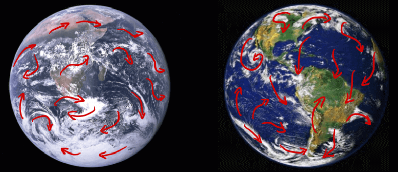
So a flow $\Phi _ 1​$ maps each point, at each time, to another point on the manifold. In other words, $\Phi _ 1​$ assigns a history and a future to where every single point on the manifold have been and will be. By the same rationale, $\Phi _ 2​$ can assign a different history and a future. To put it more intuitively, a flow is like a “cloud forecast” on earth. Each “cloud” is assigned to a certain position on the planet. Over time that assignment becomes a “flow”, hence the name. Since there is freedom to make up different versions of such forecasts (below are two versions of flow, from [giphy]), different flows can be defined.